
Aug 13, 2019 • Avik Das
My friend has recently been going through Cracking the Code Interview. I’m not a fan of any interview process that uses the types of questions in the book, but just from personal curiosity, some of the problems are interesting. One such problem was Baby Names, which I realized was a fun application of an important computer science concept.
This post assumes some computer science knowledge, namely about graphs and graph traversals. The intended audience is someone with that knowledge who wants to see an interesting application of the theory.
We want to find out what baby names were most popular in a given year, and for that, we count how many babies were given a particular name. However, different parents have chosen different variants of each name, but all we care about are high-level trends. For example, the names John, Jon and Johnny are all variants of the same name, and we care how many babies were given any of these names.
The input consists of two parts:
A set of name and count pairs.
A set of name pairs, where both names in each pair are synonyms of each other.
Note that the synonyms are:
Bidirectional, meaning if ("John", "Jon") is a synonym pair, then John is a synonym of Jon and vice versa.
Transitive, meaning if John and Jon are synonyms, and Jon and Johnny are synonyms, then John and Johnny are also synonyms, even if that last pair doesn’t appear in our input.
The output is a new set of name and count pairs, but the names have been normalized to only one representative in each set of synonyms. Any representative can be picked from each set of synonyms.
Let’s take a concrete example. Our input is:
The raw counts: ("John", 10), ("Kristine", 15), ("Jon", 5), ("Christina", 20), ("Johnny", 8), ("Eve", 5), ("Chris", 12)
The synonyms: ("John", "Jon"), ("Johnny", "John"), ("Kristine", "Christina")
One possible output is ("John", 23), ("Christina", 35), ("Eve", 5), ("Chris", 12).
When I see a problem like this, I try to visualize the data. For this problem, let’s visualize the synonyms. We have a set of names, which we can draw as a bunch of data points. We also have connections between some of the names, which we can draw as lines between connected names.
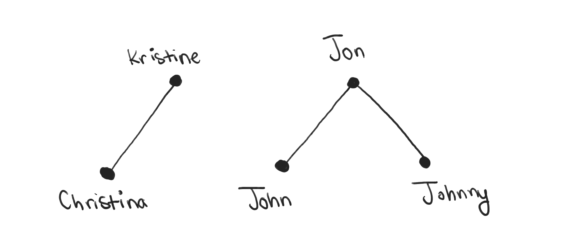
One of the properties of the lines between names is that there is no directionality of the lines. This comes from the fact that synonyms are bidirectional. Looking at the drawing, we also see that if we consider indirect connections, we’ve represented transitivity.
This is where the computer science kicks in. The above drawing represents a graph, with names as nodes and an edge between two nodes that are specified as synonyms in the input. Because of transitivity, two names are synonyms even if they’re not specified that way in the input, as long as there is some path between them.
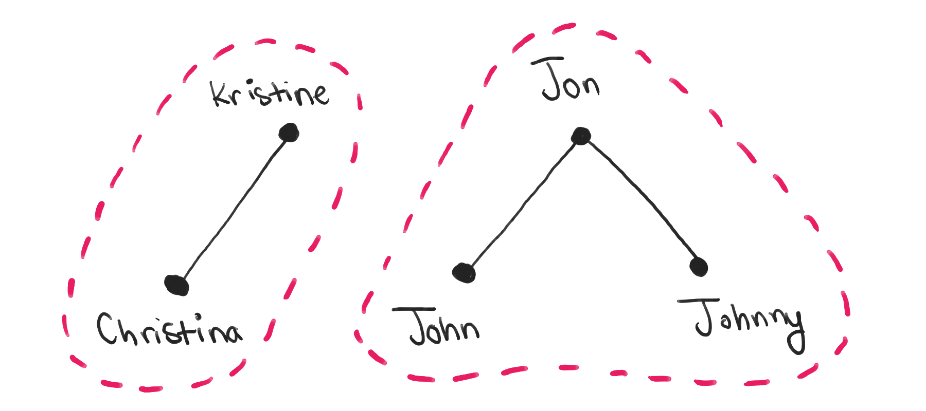
Visually, there are some interesting patterns. There seem to be clusters of names that are connected to each other, and each cluster is completely separated from each other. That makes sense: each cluster represents a set of names that are all synonyms of each other. Separate clusters represent completely different names with no relation to each other.
In computer science, these clusters are called connected components. This is the key insight: we want to find the connected components in this synonym graph and pick one node from each component as the representative name for that component.
By framing the problem in this way, we can apply standard tools to the problem. To find connected components in a graph, we go through each node in the graph and perform a graph traversal from that node to find all connected nodes. By visiting each node once, we can find each connected component.
With the problem framed in terms of connected components, the implementation is pretty straightforward. The remainder of the blog post shows one way I would approach the implementation, in case you’re also interested in seeing some code.
First, we need to represent an undirected graph. An easy way to do this is with adjacency lists, where each node points to all its neighbors. In a sense, we’re actually representing a directed graph, where the edges have a direction. We’ll just make sure the nodes at each side of an edge point to each other.
Let’s start by representing a node with a name and a list of neighbors:
class NameNode:
    def __init__(self, name):
        self.name = name
        self.adjacent_nodes = []
Next, we need to create nodes for each name in the synonyms given in the input. Note that I’ll store the nodes keyed by name so it’s easier to connect them up in the next step.
# 1. Find all unique names with synonyms
names_with_synonyms = set(name for pair in synonyms for name in pair)

# 2. Create nodes for each name in synonyms. Index the nodes by the
#    corresponding names in order to make it easy to look up the nodes.
nodes_by_name = {name: NameNode(name) for name in names_with_synonyms}
Finally, we go through each pair in the synonym set and point the corresponding nodes to each other. Because the synonym set contains pairs of names, it helps to be able to look up the corresponding nodes by name.
# 3. Add edges in for the names with synonyms
for name1, name2 in synonyms:
    node1 = nodes_by_name[name1]
    node2 = nodes_by_name[name2]

    node1.adjacent_nodes.append(node2)
    node2.adjacent_nodes.append(node1)
The next step is to actually find the connected components in this graph. As mentioned above, we want to perform some graph traversal starting at certain nodes. I’ll talk in a bit about how to choose these starting points, but let’s implement a simple breadth-first search using a queue data structure. In Python, I use collections.deque.
I won’t go through this part in very much detail, as it’s a very standard breadth-first search implementation:
from collections import deque

def nodes_in_connected_component_with(start_node):
    """
    Find all the nodes connected to the given starting node using a
    breadth-first search (BFS).
    """

    visited = set()

    frontier = deque()
    frontier.append(start_node)

    component = []
    while frontier:
        node = frontier.popleft()
        visited.add(node)
        component.append(node)

        for adjacent in node.adjacent_nodes:
            if adjacent not in visited:
                frontier.append(adjacent)

    return component
Now, we’ll go through all the nodes in the graph, performing the breadth-first search starting at each node. This will give us the nodes in the connected component containing that starting node. Once we have the nodes in that connected component, we don’t want to do a graph traversal from any of those nodes again, so we mark all of those nodes as visited.
# 4. Find connected components within the synonyms graph
components = []
visited = set()
for node in nodes_by_name.values():
    if node.name in visited:
        continue

    component = nodes_in_connected_component_with(node)
    visited.update(node.name for node in component)
    components.append(component)
The following animation visualizes this algorithm, showing the following steps:
The “Christina” node is visited, starting the first component.
A breadth-first search is performed from this node, extending the component to include “Kristine”.
At this point, no more nodes can be visited by the BFS, so we start a new component with “John”. Note that we don’t visit “Kristine” at this stage because that node has been visited as part of a previous component.
The BFS extends the new component to include “Jon”.
The BFS continues extending the component to also include “Johnny”. Now, all the nodes have been visited, so the algorithm is complete.

Finally, for each connected component, we’ll pick an arbitrary node in that component as the representative for that component. Later, given any name, we want to find the representative for the given name, so we’ll map each name in the connected component to the representative name.
# 5. Map each name to a representative of its connected component
representative_name_by_actual_name = {}
for component in components:
    representative_name = component[0].name

    for node in component:
        representative_name_by_actual_name[node.name] = representative_name
The last piece of the puzzle is to go through the original name frequencies and group the counts based on representative names. For each original name, we’ll look up to see if there is an assigned representative name. If so, we’ll add the count for the original name to the total count for the representative name. If there is no representative, that means the original name had no synonyms, and we’ll just map the original name to the original count.
# 6. Normalize counts using connected components
counts_by_representative_name = {}
for raw_name, count in raw_counts:
    representative_name = \
        representative_name_by_actual_name[raw_name] \
        if raw_name in representative_name_by_actual_name \
        else raw_name

    previous_count = \
        counts_by_representative_name[representative_name] \
        if representative_name in counts_by_representative_name \
        else 0

    counts_by_representative_name[representative_name] = \
        previous_count + count
And there we go, we have counts_by_representative_name, our new frequencies!
If you take a problem like Baby Names and try to solve it in one go, you’ll end up trying to solve too many unrelated problems at once. How do you keep running totals of the counts based on representative names? How do you follow transitive links between sets of synonyms? How do you pick one constant representative for each set of synonyms? All of these concerns end up muddled together.
Instead, the better approach is to step back and see what tools we already have to solve part of the problem. In this case, it turns out the synonyms formed a graph and we could find connected components within that graph. Then, by doing some pre-processing to transform the original problem into the graph problem, solving the graph problem using standard computer science techniques, and finally post-processing the solution into what you originally wanted, you’ve created cleaner, more understandable code.
Don’t forget your computer science fundamentals. They can come up in very interesting places!