
Backtracking is all about exploring the branches of a solution space. Photo by Brandon Green on Unsplash.
Feb 25, 2020 • Avik Das
Backtracking is all about exploring the branches of a solution space. Photo by Brandon Green on Unsplash.
In my last post, I introduced the balanced parentheses problem. The solution required trying out multiple possibilities whenever there was a choice to be made, a solution I referred to as backtracking.
If you read my graphical introduction to dynamic programming, you’ll know I frequently bring up choice as a key concept when applying dynamic programming to problems. So how do backtracking and dynamic programming differ, and when do you apply one over the other? In this post, I’ll lay out some fundamental principles to answer those questions, then explore these principles with a few examples.
Backtracking has three fundamental traits:
When faced with a choice, each possibility is explored recursively.
After trying one choice and before trying the next, the program state is restored back to exactly what it was before trying the first choice.
When it’s clear an exploration path will not lead to a viable solution, the exploration of that path stops.
Let’s see how these traits apply to the last variant of the balanced parentheses problem. First, the choice inherent to our problem was whether to treat a delimiter as an open delimiter or a close delimiter. Let’s take as an example the following delimiter pairs:
a -> A
A -> b
b -> B
We want to check if the following string is balanced:
aaAbBbAA
Because the string is small, we can see the string is balanced, as followed, using height to represent nesting:
   bB
  A  b
 a    A
a      A
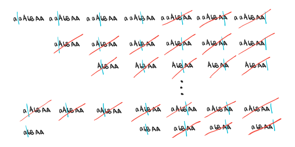
The choice occurs when the first A is encountered, and we want to know if we should use it to close the previous a or to start a new group. We can represent this choice as a tree, forking into two children whenever we have a choice. In this view, each node in the tree represents the current stack of delimiters that have yet to be closed.

In this way, the backtracking algorithm amounts to a depth-first search of the solution space. Technically, the search may be over a graph, as certain configurations may be visited multiple times. However, in this case, it’s more likely we’ll visit each configuration only once (a fact that’s detailed later in the post), making it more natural to view the algorithm as a tree search.
Notice the first important trait of backtracking: one choice can lead to another, and the resulting choices must be explored recursively. For example, if we assume the first A is an open delimiter, we now face the choice of whether b is an open or close delimiter. This leads to another choice, which would also be explored fully, and so on.
Secondly, after exploring the subtree in which A is an close delimiter, we would find that subtree does not result in a balanced string. So, we would explore the other subtree in which A is an open delimiter. But before doing so, out program state would be the same as is was before the first subtree was explored: the first aa have been consumed and we’re deciding what to do with the first A.
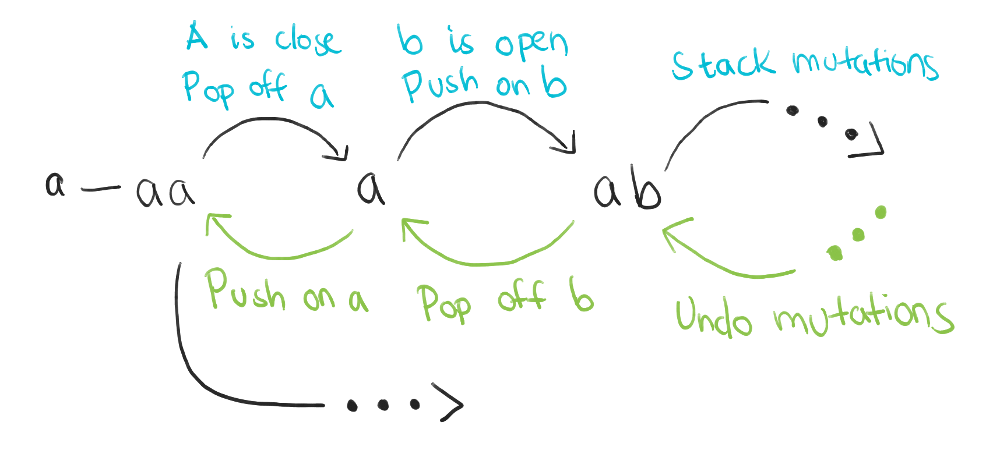
This illustrates the second trait of backtracking. Even though visiting the first subtree messed with the program state by pushing and popping items off its stack, the result after finishing the subtree exploration is as if nothing happened. In other words, each recursive tree exploration has the invariant of not changing the program state at the end of the exploration.
I see people get tripped up when they move from the iterative solution used for the second variant of the problem (a fixed set of delimiters) to a recursive solution for the third variant (user-provided delimiters). Because they are used to mutating a stack across iterations, they have trouble reconciling the mutation with recursion. But, if you maintain the invariant above, you can still mutate a single stack across recursive calls! Just make sure the stack is the same by the end of each function call!
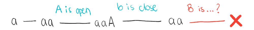
Let’s say the algorithm decides to try the following sequence of choices:
The first A is an open delimiter. This leaves us with a stack consisting of aaA and the remainder of the string as bBbAA.
The subsequent b is a close delimiter. This leaves the stack as aa (since the A just got closed) and the remainder of the string as BbAA.
But now, the algorithm is stuck because the following B can only be a close delimiter and it has nothing to close. At this point, the rest of the string doesn’t have to be processed, and the subtree starting with the sequence of decisions above no longer needs to be explored further.
In a similar vein, you also terminate once you’ve found one valid solution, as you don’t need to keep searching the rest of the solution space.
Terminating the exploration of part of the solution space is the third trait of backtracking, and it can lead to substantial performance gains.
Given these principles, how to backtracking and dynamic programming relate? It turns out both are related, and certain backtracking problems will use dynamic programming in their implementation. But the two are still separate.
Backtracking is typically used for a search problem, in which you want to find a single solution that works, out of many possible candidates. For example, in the balanced parentheses problem, it’s sufficient to find one balanced configuration, even if there are multiple. Furthermore, early termination means you don’t explore all the smaller subproblems if you can eliminate them early on.
In the bottom-up approach to dynamic programming, you start with smaller subproblems, solving them early so they’re available when you need them later. This is useful when you’ll have to solve all the subproblems eventually, like in the seam carving example I discussed.
However, when searching for a single solution, you probably don’t want to search everything! This actually came up in the change making problem I discussed earlier, where we used the top-down approach (memoization) instead of the bottom-up approach to solve the problem.
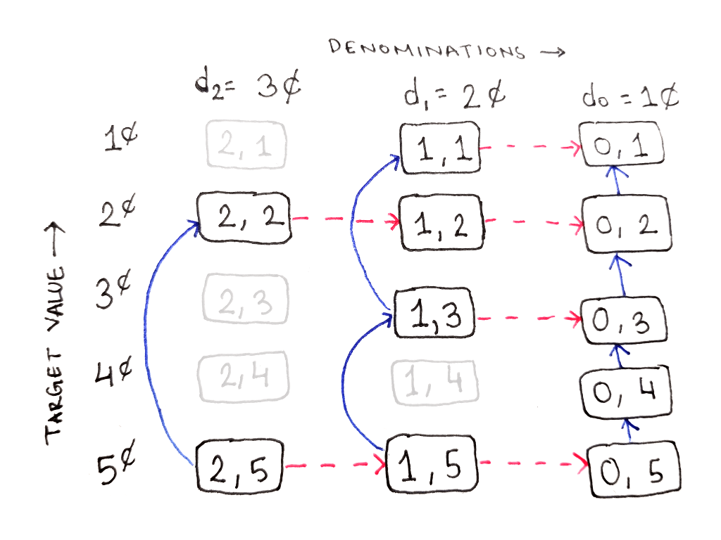
The change making problem still was concerned with finding the total number of valid configurations of coins. But, if the problem was to find one valid configuration, then backtracking with memoization would be a good fit.
With dynamic programming, the first step was to define a recurrence relation, a recursive function with an important property:
The function should be identifiable by some integer inputs. This will allow us to associate the inputs with already-computed results, as well as evaluate the function in a defined order.
The ability to associate subproblems with integers meant the node for each subproblem was easy to represent: one subproblem is one list of integers. Now, think about the inputs to each recursive call in the balanced parentheses problem. Not only is there the remainder of the string, but there’s a stack of open delimiters. How do you even represent these inputs as integers?!
(Okay, you can represent them as integers, but in practice, you don’t really want to.)
So backtracking without dynamic programming is useful when either:
It’s not easy to tell if you’ve visited a particular configuration before.
Or, you don’t expect to visit the same configurations multiple times because the solution space is too large.
In these cases, you forgo the memoization or the table structure that’s integral to dynamic programming.
Backtracking is a useful technique for solving search problems, with a few fundamental properties:
Choices are explored recursively.
Program state is restored after each explored branch.
The algorithm can terminate early depending on what is found.
These properties can be compatible with dynamic programming, and indeed, dynamic programming can be a tool to implement a backtracking algorithm. However, the two are separate and are used for different classes of problems.
In later posts, I plan to visit some more complicated backtracking problems to see how they utilize the properties above.