
Jul 21, 2020 • Avik Das
After my recent post on getting started with WebGL, it’s time to move onto 3D rendering. It turns out, I had most of the OpenGL concepts in place already. But, what I needed to understand was what format OpenGL needed my data in order to get the results I wanted.
In this post, I’ll implement the bare minimum changes needed to implement useful 3D rendering. This entails:
Specifying 3D positions for a mesh, along with colors for the different faces. Colors let us see the different faces, without having to implement shading yet.
Perspective projection.
Rotation and animation. While not strictly necessary, some rotation is the only way to see the different sides of the model. And, understanding how the rotation works is crucial for implementing a camera in the future.
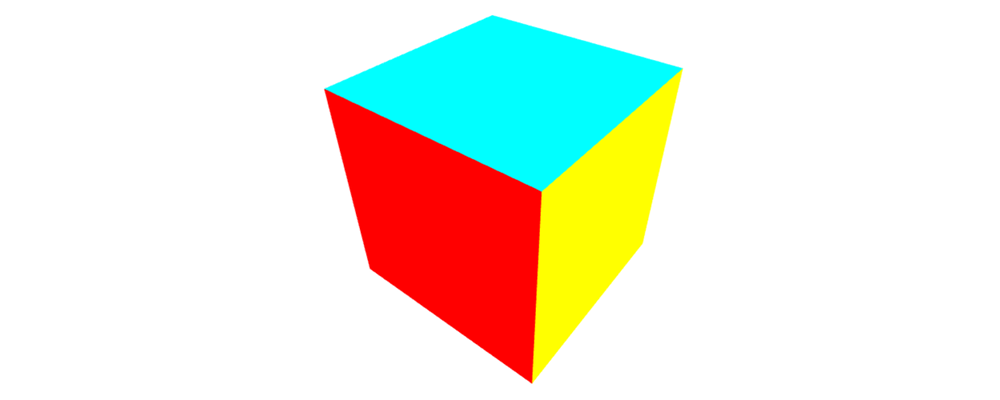
Here’s what we’ll make:
I want to be clear about the audience for this post. This post is aimed towards people like myself, who understand 3D rendering concepts (homogeneous coordinates, matrix transformations, etc.) but need to connect those concepts to the OpenGL/WebGL APIs.
Even though OpenGL leaves it up to developers to implement how rendering is done, some parts of the rendering are set in stone. Application code can specify what vertices to render, and how pixels look on screen, but OpenGL automatically decides which pixels to even paint based on some fixed code known as rasterization.
Because we’ll actually be creating a more complicated model, we want two useful features enabled:
Depth tests. This ensures triangles closer to the viewer block those farther away.
Back-face culling. This is not strictly necessary, but is nice as an optimization to avoid drawing triangles that are facing away from the viewer. Useful for not rasterizing triangles that will never be seen on a completely closed model. Note: you don’t want this for open meshes, or ones with transparency.
These two features can be enabled at any time, but since we always want them for our renderer, we can enable them right as soon as we get the GL rendering context:
 const gl = canvas.getContext('webgl');

+gl.enable(gl.DEPTH_TEST);
+gl.enable(gl.CULL_FACE);
(Here’s the page for the glEnable call, specifically for the OpenGL version WebGL 2.0 is based on.)
With the depth test enabled, we also need to clear the depth buffer before rendering. Otherwise, older values in the depth buffer might carry over to the new render. Do this right before the glDrawArrays call.
+gl.clear(gl.COLOR_BUFFER_BIT | gl.DEPTH_BUFFER_BIT);
 gl.drawArrays(gl.TRIANGLES, 0, 3 * 2 * 6);
If you don’t enable these features, your model may look like this:

The vertex shader actually generates 3D points (really 4D in homogeneous coordinates) to rasterize. That means your input to the vertex shader can be anything that you can convert into a 3D point, as long as you have one set of inputs for every point you’ll generate.
For a basic mesh, we’ll want a 3D position (actually 3D, not 4D, because the w-coordinate will always be 1) and a color. The latter is just nice to give the various triangles their own colors, and it nicely demonstrates how we can feed two separate pieces of information into the shader. Let’s update our vertex shader to include the input color, then pass along that input color to the fragment shader:
 attribute vec3 position;
+attribute vec3 inputColor;
 varying vec4 color;

 void main() {
   gl_Position = vec4(position, 1);
-  color = gl_Position * 0.5 + 0.5;
+  color = vec4(inputColor, 1);
 }
To feed in two inputs, we have two (out of many) options:
Create separate Vertex Buffer Objects (VBOs) for each input. Remember that a VBO is essentially a sequence of bytes. This is useful if the inputs change with different frequency during the program execution, like if one is static and another changes every frame.
Create a single VBO with both pieces of information interleaved.
As we’ll see soon, we’ll keep both the base position and the color constant throughout the program, so the second option makes sense. So now, we can specify both pieces of data in a single Float32Array.
const vertexData = new Float32Array([
  // Six faces for a cube.
  // Each face is made of two triangles, with three points in each triangle.
  // Each pair of triangles has the same color.

  // FRONT
  /* pos = */ -1, -1,  1, /* color = */ 1, 0, 0,
  /* pos = */  1, -1,  1, /* color = */ 1, 0, 0,
  /* pos = */  1,  1,  1, /* color = */ 1, 0, 0,

  /* pos = */ -1, -1,  1, /* color = */ 1, 0, 0,
  /* pos = */  1,  1,  1, /* color = */ 1, 0, 0,
  /* pos = */ -1,  1,  1, /* color = */ 1, 0, 0,

  // And so on for the other five faces...
  // See the source code for this post to see the full mesh
  // ...
]);
The question is: where should we place the points? After all, where is the camera? The trick is OpenGL wants the points in a specific coordinate system, which I’ll talk about below. But, our vertex shader is the one generating points. That means we can place the input points where they’re useful for modeling purposes (e.g. around the origin like I’ve done), and the vertex shader can move them to a location the OpenGL rasterizer will actually recognize.
As an aside, you need to be careful about which order you specify the points for each triangle. Because we turned on back-face culling, you want to specify the points in counter-clockwise order when viewed from the front.
Finally, we can now connect both pieces of data, which are interleaved in a single byte sequence, to their corresponding shader inputs:
Still create only one buffer on the GPU. Continue to bind it ot the GL_ARRAY_BUFFER for sending data to the buffer.
Grab a handle to the position variable in the vertex shader. Point that handle to the buffer, with a stride of 24 and an offset of 0. This means the relevant data is available every 24 bytes (floats are 4 bytes), starting at the first byte.
Repeat with the inputColor variable. This time, use the same stride but an offset of 12.
The code looks like this:
const vertexBuffer = gl.createBuffer();
gl.bindBuffer(gl.ARRAY_BUFFER, vertexBuffer);
gl.bufferData(gl.ARRAY_BUFFER, vertexData, gl.STATIC_DRAW);

const positionAttribute = gl.getAttribLocation(program, 'position');
gl.enableVertexAttribArray(positionAttribute);
gl.vertexAttribPointer(positionAttribute, 3, gl.FLOAT, false, 24, 0);

const colorAttribute = gl.getAttribLocation(program, 'inputColor');
gl.enableVertexAttribArray(colorAttribute);
gl.vertexAttribPointer(colorAttribute, 3, gl.FLOAT, false, 24, 12);
We’ll also need to tell the glDrawArrays call to actually render the correct number of triangles:
-gl.drawArrays(gl.TRIANGLES, 0, 3);
+gl.drawArrays(gl.TRIANGLES, 0, 3 * 2 * 6);
At this point, your program will show nothing, because the way we convert the 3D input point into a 4D gl_Position means we’re essentially inside the cube looking out. Back-face culling means the inner sides of the cube faces aren’t visible. If you turn off the culling, you’ll see a single blue square.
(Note: I’m deliberately not introducing another concept, known as an Element Buffer Object or EBO. While this concept is useful for sharing points across multiple vertices, I want to introduce only the necessary concepts right now.)
Before fixing the shader to place points in a visible location, I want to take a detour and start re-rendering the model every frame. The reason is, to view every part of the cube, we want to rotate it over time. That means we can no longer render it in a fixed orientation and leave it that way.
This part is pretty easy: just wrap the glClear and glDrawArrays calls (the two parts that are actually doing the drawing) inside a function that is called by requestAnimationFrame.
requestAnimationFrame(t => loop(gl, t));

function loop(gl, t) {
  gl.clear(gl.COLOR_BUFFER_BIT | gl.DEPTH_BUFFER_BIT);
  gl.drawArrays(gl.TRIANGLES, 0, 3 * 2 * 6);

  requestAnimationFrame(t => loop(gl, t));
}
Note the t parameter will be useful for automatically rotating the cube in the future.
There’s nothing WebGL or OpenGL-specific about this change. It’s common to do this in web animation code.
The last step is to take the input positions, specified in a way that’s convenient for modeling, and output positions OpenGL can actually rasterize correctly. That means generating final positions that are in clip space, which is basically a 3D cube ranging from -1 to 1 in each direction. Any point inside this cube will be rasterized.
However, there are actually a few related concepts at play:
Vertex shader input data. The data here can be in any form, and doesn’t even have to be coordinates. However, in practice, the input data is typically composed of 3D points in some coordinates that are easy for modeling, in which case the points are considered to be in model space.
Clip space. This is the output of the vertex shader, in homogeneous coordinates.
Normalized Device Coordinates. The same points in clip space, but converted from homogeneous coordinates to 3D Cartesian coordinates by doing a w-divide. Only points within a 2×2×2 cube centered around the origin (between -1 and 1 on all axes) will be rendered.
Screen space. These are 2D points where the origin, which used to be in the center of the space, is the bottom-left of the canvas. The z-coordinate is only used for depth sorting. These are the coordinates that end up being used for rasterization.
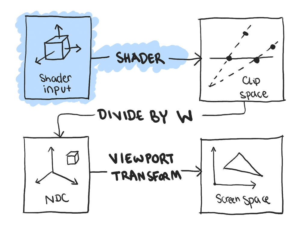
The reason for my breakdown is many tutorials talk about model, world, and view space alongside clip space, NDC and screen space. But it’s important to realize that everything before clip space is up to you. You decide what the input data looks like and how it gets converted into clip space. That probably means specifying the inputs in model space, then sequentially applying the local and camera transformations. But if you want to understand the OpenGL APIs, it’s important to first understand what’s under your control and what the OpenGL provides for you.
Here’s the cool part: if you wanted, you could pre-compute the coordinates directly in clip space and your vertex shader would just pass along the input positions to OpenGL. This is exactly what our first demo did! But, doing so per-frame is expensive, since the transformations we usually want to do (matrix multiplications) are much faster on the GPU.
To convert from the model space coordinates specified in the VBO to clip space, let’s break up apart the transformation into two parts:
A model to world space transformation.
A perspective projection transformation.
This breakdown works for our purposes, because we’ll rotate the cube over time will leaving the perspective projection the same. In real-world applications, you’d slot in a camera (or view) transformation in between the two steps to allow for a moving camera without having to modify the entire world.
Start by adding two uniform variables to the shader. Remember that a uniform is a piece of input data that is specified for an entire draw call and stays constant over all the vertices in that draw call. In our case, at any given moment, the transformations are the same for all the vertices of the triangles that make up our cube.
The two variables represent the two transformations, and therefore are 4×4 matrices. We can use the transformations by converting the input position into homogeneous coordinates, then pre-multiplying by the transformation matrices.
 attribute vec3 position;
 attribute vec3 inputColor;
+uniform mat4 transformation;
+uniform mat4 projection;
 varying vec4 color;

 void main() {
-  gl_Position = vec4(position, 1);
+  gl_Position = projection * transformation * vec4(position, 1);
   color = vec4(inputColor, 1);
 }
Let’s populate one of the two matrices above, namely the projection matrix. Remember that, because of the way our vertex shader is set up, the projection matrix will take points in world space (where the input points end up after the model transformation) and put them into clip space. That means the projection matrix has two responsibilities:
Make sure anything we want rendered gets put into the the 2×2×2 cube centered around the origin. That means every vertex that we want rendered should be have coordinates in the range of -1 to 1.
If we want perspective, set up the w-coordinate so that dividing by it performs a perspective divide.
I won’t go into the math of the perspective projection matrix, as it’s covered in other places. What’s important is we’ll define the matrix in terms of some parameters, like the distance to the near and far clipping panes, and the viewing angle. Let’s look at some code:
const f = 100;
const n = 0.1;
const t = n * Math.tan(Math.PI / 8);
const b = -t;
const r = t * gl.canvas.clientWidth / gl.canvas.clientHeight;
const l = -r;

const projection = new Float32Array([
    2 * n / (r - l),                 0,                    0,  0,
                  0,   2 * n / (t - b),                    0,  0,
  (r + l) / (r - l), (t + b) / (t - b),   -(f + n) / (f - n), -1,
                  0,                 0, -2 * f * n / (f - n),  0,
]);
To make sense of this matrix, notice the following:
Most importantly, matrices in OpenGL are defined in column-major order. That means the first four values above are actually the first column. Similarly, every fourth value contributes to a single row, meaning the bottom-most row is actually (0, 0, -1, 0) above.
The first three rows use the bounds defining the perspective transform to bring in the x, y and z-coordinates into the correct range.
The last row multiplies the z-coordinate by -1 and places it into the output w-coordinate. This is what causes the final “divide by w” to scale down objects that have a more negative z-coordinate (remembering that negative z values point away from us). If we were doing an orthographic projection, we would leave the output w-coordinate as 1.
Now, that we have a matrix, in the correct format, we can associate it with the variable in the shader. This works somewhat similarly to how an array is associated with an attribute variable. However, because a uniform contains essentially one piece of data to be shared by all vertices (as opposed to one piece of data per vertex), there’s no intermediate buffer. Just grab a handle to the variable and send it the data.
const uniformP = gl.getUniformLocation(program, 'projection');
gl.uniformMatrix4fv(uniformP, false, projection);
Make sure to do this outside the loop function. We won’t change the projection throughout the program execution, so we only need to send this matrix once!
A traditional projection matrix assumes points in “view space”, that is in the view of a camera. To keep things simpler, we’ll assume the camera is at the origin and looking at the negative z direction (which is what view space essentially is). So now, the goal is to transform the shader input positions into points that are within the viewable area defined by the perspective projection’s field of view and clipping planes.
I chose the following transformations, in the following order:
The choice was pretty arbitrary, but this resulted in a cube that had most sides visible (the very back face never came into view), filled up most of the canvas, and was relative easily to calculate by hand.
I took the usual transformation matrices for these transformations (you can find them online), multiplied them in reverse order, and finally transposed them to get them into column-major order. I defined the matrices with some variables so I could easily vary the angle of rotation:
const uniformT = gl.getUniformLocation(program, 'transformation');

function loop(gl, t) {
  const a = t * Math.PI / 4000;
  const c = Math.cos(a);
  const s = Math.sin(a);
  const x = 2;
  const tz = -9;

  const transformation = new Float32Array([
     c * x,  s * s * x, -c * s * x, 0,
         0,      c * x,      s * x, 0,
     s * x, -c * s * x,  c * c * x, 0,
         0,          0,         tz, 1,
  ]);

  gl.uniformMatrix4fv(uniformT, false, transformation);

  gl.clear(gl.COLOR_BUFFER_BIT | gl.DEPTH_BUFFER_BIT);
  gl.drawArrays(gl.TRIANGLES, 0, 3 * 2 * 6);
}
Notice that the model transformation matrix is defined inside the loop function, allowing the use of the time parameter to define the angle of rotation. Otherwise, associating the resulting matrix with the shader variable is exactly the same as before.
And with all that, we have our rotating cube! (I put it behind a play button to prevent the animation from using up your battery while you read the article.)
The entire code is embedded within this post. You’ll find a large portion of the code is defining the vertex shader input data.
Now that I have a basic 3D rendering pipeline set up in OpenGL, I can start building on top of it. Here are some areas I’ll visit next.
I plan to do a follow up with indexed drawing, in which we can reference the same vertex multiple times in the same mesh. That saves space and computation when defining the mesh, and promotes consistency within the model.
In legacy OpenGL, you were forced to use the shading models OpenGL provided. In modern OpenGL, you decide how to shade your models in the fragment shader code. I won’t go into the topic in this post, but basically, you output normal vectors from your vertex shader, which get interpolated across fragments and passed into the fragment shader. Then, in the fragment shader, you use the passed in normal to implement a shading model such as Phong shading.
Admittedly, generating the various transformation matrices is pretty painful to do by hand. However, it was important for me to understand how the theory (which I already understand) maps to the data format OpenGL expects. Now that I understand the connection, I’ll certainly use glMatrix going forward.
The manual approach is especially important for the mesh definition, where I could have used an object loader library. I’m personally interested in procedurally generating a mesh, so it’s important I understand what kind of data I need to generate.