Apr 15, 2019 • Avik Das
I’ve been helping a friend understand dynamic programming (DP for short), so I’ve been on the lookout for good resources. The topic is covered all across the web, but I found many of them focused on the code, and not enough on the beautiful visualizations that shed light into how DP works.
In this post, I present a highly visual introduction to dynamic programming, then walk through three separate problems utilizing dynamic programming.
The classic introductory problem in teaching DP is computing the Fibonacci numbers. As a reminder, the Fibonacci numbers are a sequence starting with 1, 1 where each element in the sequence is the sum of the two previous elements:
\[1, 1, 2, 3, 5, 8, 13, 21, ...\]The canonical recursive formula for the $n$th element in the sequence is:
\[\begin{aligned} F_0 &= 1 \\ F_1 &= 1 \\ F_n &= F_{n-1} + F_{n-2} \\ \end{aligned}\]This translates cleanly into code, presented here using Python:
def fib(n):
    # Ideally check for negative n and throw an exception
    if n == 0: return 1
    if n == 1: return 1
    return fib(n - 1) + fib(n - 2)
The problem is, as the input $n$ gets larger, the function gets really slow. Timing the function by running it 100 times for the inputs 10, 20 and 30 give the following times:
>>> import timeit
>>> timeit.timeit('fib(10)', number=100, globals=globals())
0.01230633503291756
>>> timeit.timeit('fib(20)', number=100, globals=globals())
0.3506886550458148
>>> timeit.timeit('fib(30)', number=100, globals=globals())
34.2489672530209
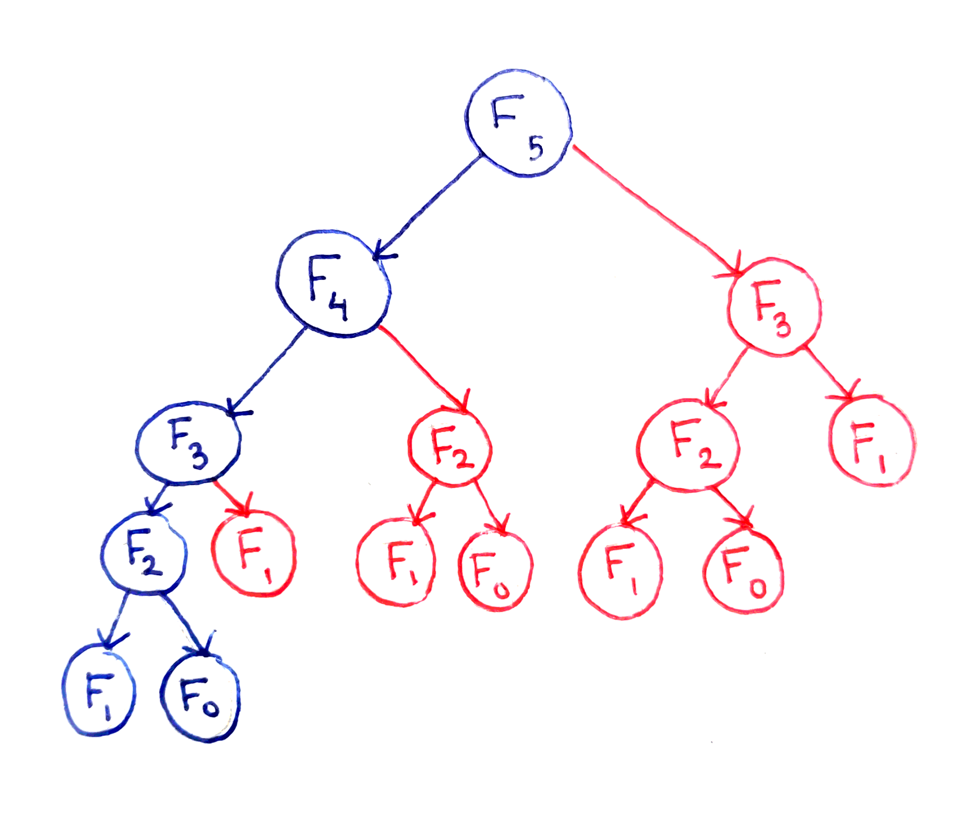
Yikes! Going from 10 to 20 causes the run time to jump by a factor of 30, but going from 20 to 30 corresponds to a jump of 100. To find out why this is, let’s look at the call tree of this implementation. Suppose we want to compute $F_5$. The following diagram shows the computation of the main problem depends on subproblems.
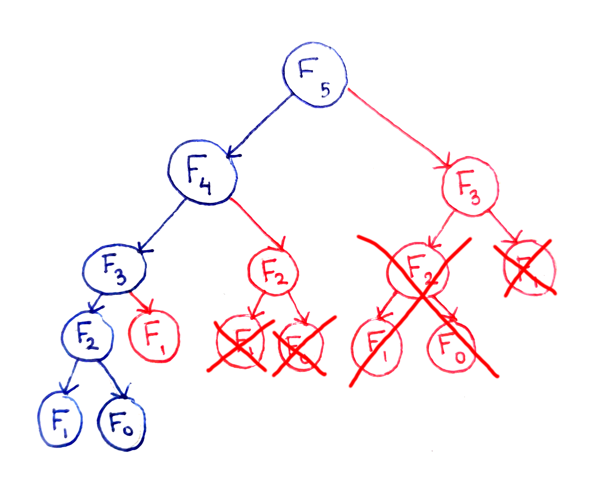
The fundamental issue here is that certain subproblems are computed multiple times. For example, $F_3$ is computed twice, and $F_2$ is computed three times, despite the fact they will produce the same result each time. I won’t go into the full analysis of the run time, but this algorithm ends up with a run time that’s exponential in $n$.
This is the hallmark of a problem suitable for DP. Dynamic programming helps us solve recursive problems with a highly-overlapping subproblem structure. “Highly-overlapping” refers to the subproblems repeating again and again. In contrast, an algorithm like mergesort recursively sorts independent halves of a list before combining the sorted halves. When the subproblems don’t overlap, the algorithm is a divide-and-conquer algorithm.
One way to avoid re-calculating the same subproblems again and again is to cache the results of those subproblems. The technique is:
If the cache contains the result corresponding to a certain input, return the value from the cache.
Otherwise, compute the result and store it in the cache, associating the result with the input that generated it. The next time the same subproblem needs to be solved, the corresponding result will already be in the cache.
It’s easy to transform the straightforward recursive algorithm into a memoized one by introducing a cache.
def fib(n, cache=None):
    if n == 0: return 1
    if n == 1: return 1

    if cache is None: cache = {}
    if n in cache: return cache[n]

    result = fib(n - 1, cache) + fib(n - 2, cache)
    cache[n] = result
    return result
Let’s time this version:
>>> timeit.timeit('fib(10)', number=100, globals=globals())
0.0023695769486948848
>>> timeit.timeit('fib(20)', number=100, globals=globals())
0.0049970539985224605
>>> timeit.timeit('fib(30)', number=100, globals=globals())
0.013770257937721908
Ok, that looks linear! But what about the space complexity? Well, to compute $F_n$, we need to compute $F_{n-1}$, $F_{n-2}$, all the way down to $F_0$. That’s $O(n)$ subproblems that are cached. This means we’ll use $O(n)$ space.
Can we do better? In this case, yes!
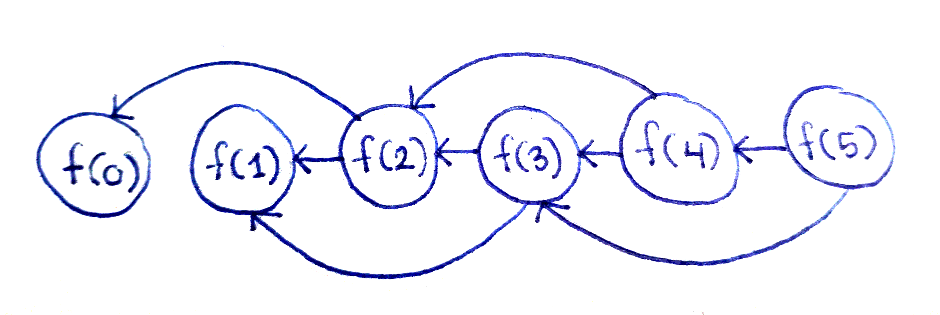
Let’s take a look at the call tree diagram again, but this time, let’s only show each subproblem once. This means that if two distinct problems depend on the same subproblem, the subproblem will have two arrows pointing to it:
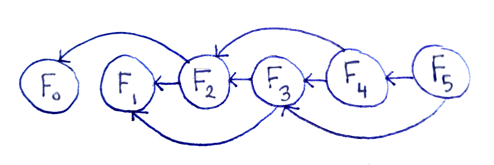
This representation is useful for a number of reasons. First, we see that there are $O(n)$ subproblems. Second, we can see the digram is a directed acyclic graph (or DAG for short), meaning:
There are vertices (the subproblems) and edges between the subproblems (dependencies).
The edges have a direction, since it matters which subproblem for every connected pair is the dependent one.
The graph has no cycles, meaning there must not be a way to start at one subproblem, then end up at that same subproblem just by following the arrows. Otherwise, we would end up in a situation where, to calculate one subproblem, we’d need to first calculate itself!
DAGs have the property of being linearizable, meaning that you can order the vertices so that if you go through the vertices in order, you’re always following the direction of the arrows. Practically, this means we can order our subproblems so that we always have the result of a subproblem before it’s needed by a larger subproblem. For Fibonacci, this order of subproblems is simply in order of increasing input, meaning we compute $F_0$, then $F_1$, then $F_2$ and so on until we reach $F_n$. This order is apparent from the diagram above.
The DAG representation also shows each subproblem depends on the two immediately preceding subproblems and no others. If you’re computing $F_m$, you only need the results of $F_{m-1}$ and $F_{m-2}$. And, if you were computing the subproblems in the order described above, you can throw away values you no longer need.
Now, we have an algorithm we can implement:
Store $F_0$ and $F_1$ (both simply 1) in local variables. At each point, these two variables will represent the last two Fibonacci numbers, as we’ll need to refer to them to calculate the next Fibonacci number.
Work your way up from $i = 2$ to $i = n$, calculating $F_i$. Each calculation only depends on $F_{i-1}$ and $F_{i-2}$, so after you’re done, you can throw away $F_{i-2}$, as you’ll never use it again. To throw away the value, update the local variables to store only $F_{i-1}$ and $F_i$ for the next iteration.
In Python:
def fib(n):
    a = 1  # f(i - 2)
    b = 1  # f(i - 1)
    for i in range(2, n + 1):  # end of range is exclusive
        # the old "a" is no longer accessible after this
        a, b = b, a + b

    return b
If you time this version, you’ll find it runs in linear time again. Additionally, because we only keep around exactly two previous results at each point, this version takes constant space. That’s a huge decrease from our previous attempts!
Because the way we approach this problem involved solving “smaller” subproblems in order to build up to bigger ones, this approach is known as the bottom-up approach.
Now that we have a framework for solving recursive problems with highly-overlapping subproblems, let’s apply this framework to a more complicated problem. In the House Robber Problem, you are a robber who has found a block of houses to rob. Each house $i$ has a non-negative $v_i$ worth of value inside that you can steal. However, due to the way the security systems of the houses are connected, you’ll get caught if you rob two adjacent houses. What’s the maximum value you can steal from the block?
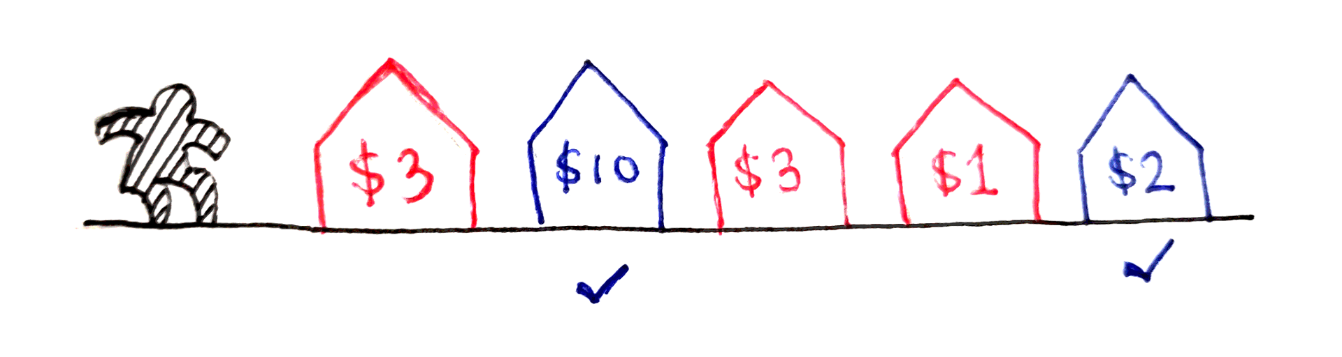
As an example, if the values of the houses are $3, 10, 3, 1, 2$, then the maximum value you can steal is $12$, by stealing from the second and fifth houses. Notice that, even though you can steal from every other house, it’s better in this case to skip two houses in a row.
The absolutely crucial first step in solving a dynamic programming problem is identifying the subproblems.
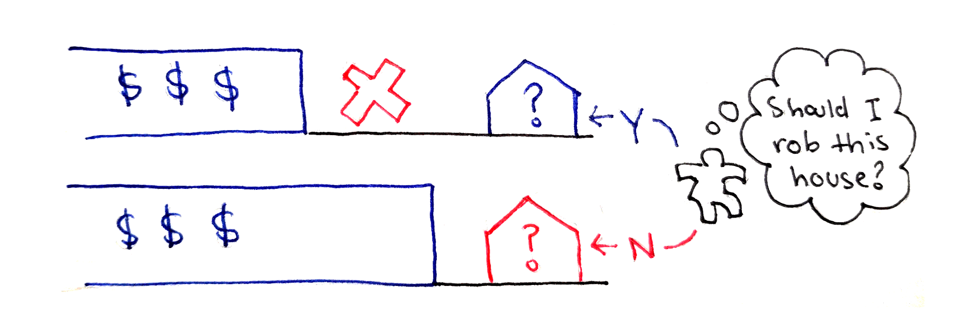
Whenever you encounter a house $i$, you have two choices:
Steal from house $i$, but then you have to maximize the stolen value up to house $i-2$, because house $i-1$ is no longer an option. In this option, you add $v_i$ to your running total.
Don’t steal from house $i$, in which case you’re free to maximize the stolen value up to house $i-1$, since that house is an option. In this option, you add nothing to your running total.
Whichever choice gives you a higher value is what you want to choose.
To formalize the above intuition, we must clearly define a function with the following properties:
The function should be identifiable by some integer inputs. This will allow us to associate the inputs with already-computed results, as well as evaluate the function in a defined order.
The solution you’re trying to find needs to be easily extracted from this function. Otherwise, the function doesn’t actually help us find the desired solution.
The function should depend on itself.
This function is known as a recurrence relation because it depends on itself.
For the House Robber Problem, the intuition above translates to the following recurrence relation. Define $f(i)$ to be the maximum value that can be stolen if only stealing from houses $0$ to $i$.
\[\begin{aligned} f(i) &= \max \begin{cases} f(i - 2) + v_i \\ f(i - 1) \\ \end{cases} \end{aligned}\]The solution we ultimately want is simply $f(n - 1)$, where $n$ is the number of houses on the block (assuming the houses are 0-indexed).
With the recurrence relation written out, we draw out the DAG for the problem. Notice it looks exactly the same as the DAG for Fibonacci. Each subproblem $f(i)$ depends on only the two previous subproblems $f(i-1)$ and $f(i-2)$. Additionally, there are $n$ subproblems: $f(0), f(1), …, f(n-1)$. That means we can solve this problem in $O(n)$ time, and in $O(1)$ space by computing the subproblems in order of increasing index, storing only the last two values at any given time.
def house_robber(house_values):
    a = 0  # f(i - 2)
    b = 0  # f(i - 1)
    for val in house_values:
        a, b = b, max(b, a + val)
    return b
As the DAG predicted, the implementation is almost the same as the one for Fibonacci, except the previous two values are combined in a different way.
Both of the previous problems have been “one-dimensional” problems, in which we iterate through a linear sequence of subproblems. The next problem has a “two-dimensional” structure.
The Change Making Problem asks what is the fewest number of coins you can use to make a certain amount, if you have coins of a certain set of denominations. You can use any quantity of each denomination, but only those denominations. Call these denominations $d_i$ and the amount to make $c$.
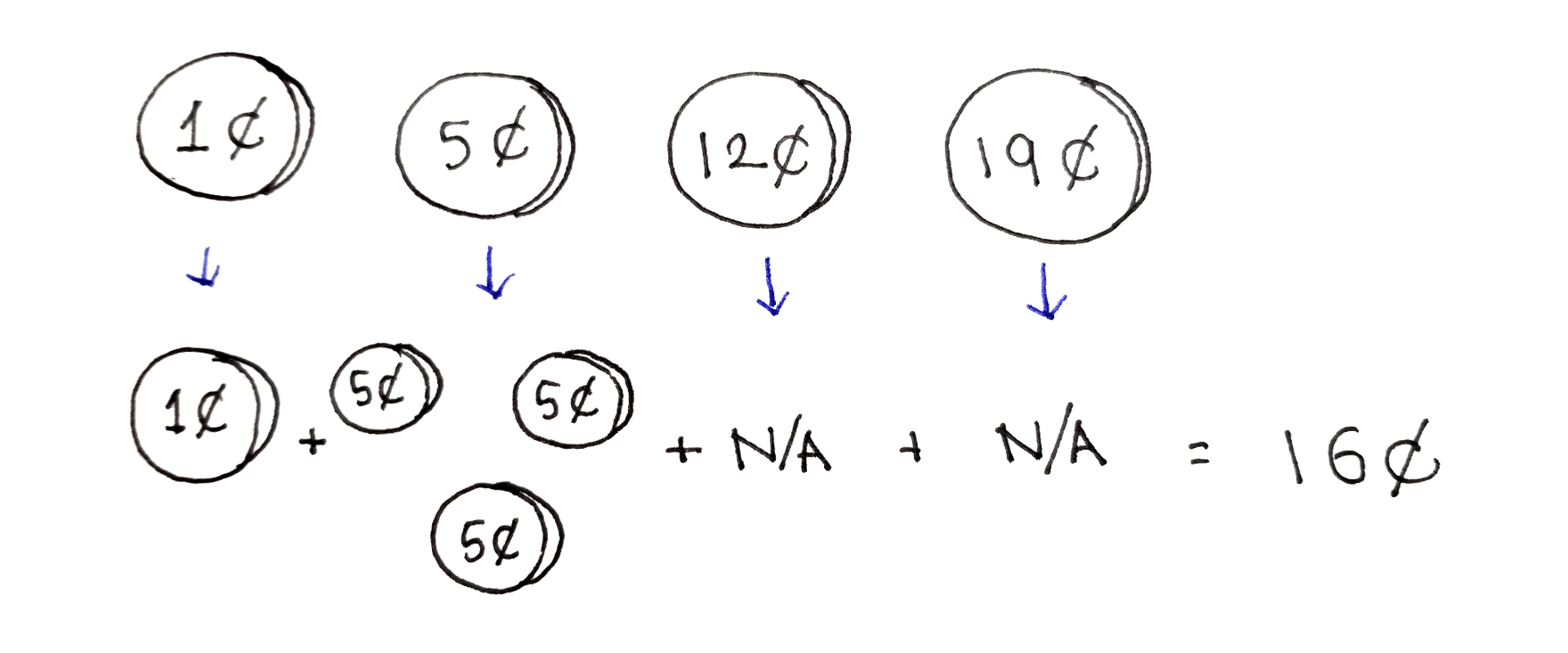
For example, suppose we have denominations 1¢, 5¢, 12¢ and 19¢, and we want to make 16¢. The fewest number of coins we can use is $4$: three 5¢ coins and one 1¢ coin. Notice it’s not always best to use the largest coin available to us, because using the 12¢ coin means using a total of $5$ coins: one 12¢ coin and four 1¢ coins.
A couple of observations right off the bat:
We can assume all the denominations are unique. Technically, this restriction is not necessary, but that makes the problem easier to reason about.
We can assume the denominations are given in increasing order of value. We could sort the denominations, but again, not having to worry about the order makes reasoning about the problem easier.
The first denomination must be $1$. Only then can every positive value be represented as a combination of the given denominations.
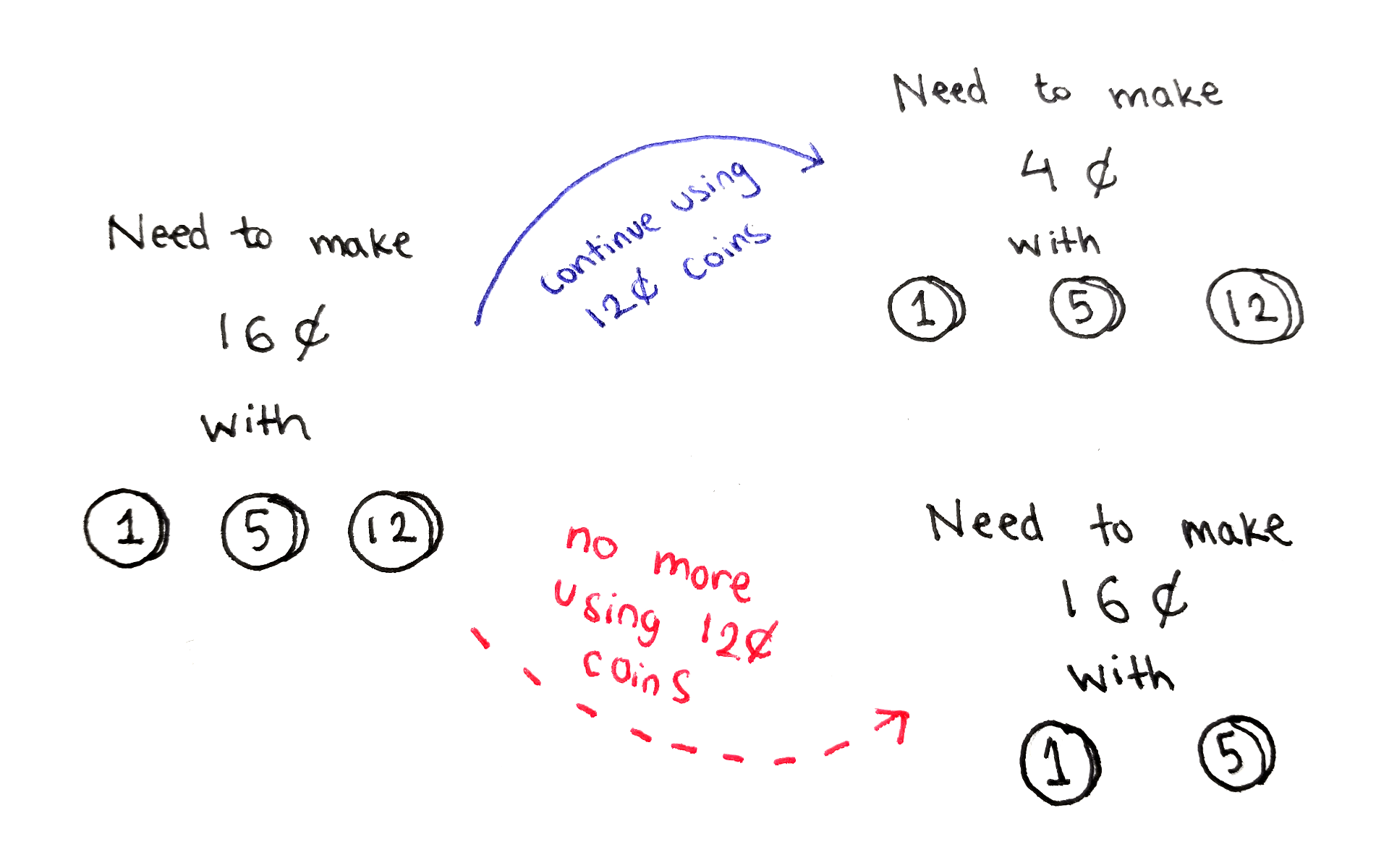
At any given point in the algorithm, we will consider a subset of the denominations, and the amount we want to add up to. This gives us two choices:
Use one coin of the highest denomination. This decreases the target amount, and we can try to reach the new target amount using the same denominations. This gives us a chance to use the same highest denomination again. If we take this choice, the number of coins used goes up by one.
Don’t use any coin of the highest denomination. Now we try to reach the same target amount, but with all but that denomination. We take this choice when we’re done with that highest denomination and want to move onto the next one. If we take this choice, the number of coins used stays the same.
Whichever choice leads to the smallest number of coins is the optimal one.
Note that we may not be able to take both choices in every situation. For example, when there is only one denomination left to consider, we have to use coins of that denomination. Likewise, when the current denomination is larger than the target value, we have to stop using that denomination.
The function we want to define needs two inputs: the subset of denominations we are allowed to use, and the target value to reach. Because we’re considering denominations in decreasing order, and all the denominations are in increasing order, we only need a single integer to represent which denominations are being considered. For example, the integer $i$ means we will only consider denominations $d_0, d_1, …, d_i$ and not the ones afterwards.
With these two inputs, we can define a function $f(i, t)$, representing the minimum number of coins needed to represent $t$ as a combination of denominations up to $d_i$. The recurrence relation is:
\[\begin{aligned} f(i, t) &= \min \begin{cases} f(i, t - d_i) + 1 \\ f(i - 1, t) \\ \end{cases} \end{aligned}\]The final answer we want corresponds to $f(n - 1, c)$, where $n$ is the number of denominations we originally were given, and $c$ is the original target value.
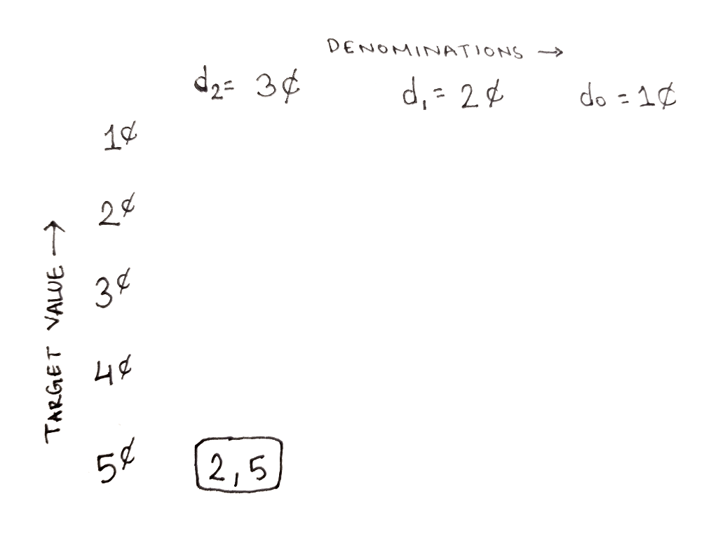
Because our recurrence relation has two integer inputs, we can lay out our subproblems as a two-dimensional table, with the first input (which denominations we will consider) indexing into the table along the horizontal axis, and the second input (the target value) indexing into the table along the vertical axis.
The exact links depend on the denominations that are available. In the example below, there are three denominations: $d_2 = 3$, $d_1 = 2$ and $d_0 = 1$, arranged in decreasing value from left to right. The final target value is $5$, but all intermediate values are present in decreasing order from bottom to top. Thus, the answer we want is at the bottom-left of the table.
The DAG for this problem is a bit complicated, so we’ll build it up one step at a time. First, let’s define the two-dimensional structure of the graph and show where the desired solution is. Each cell is indexed by two numbers: $(i, t)$, where $i$ represents the index of the largest denomination being considered and $t$ represents the current target value.
From this cell, both of our choices are available to us. Either we can move up the same column by using one coin of the highest denomination, or move one column to the right by disregarding that denomination:
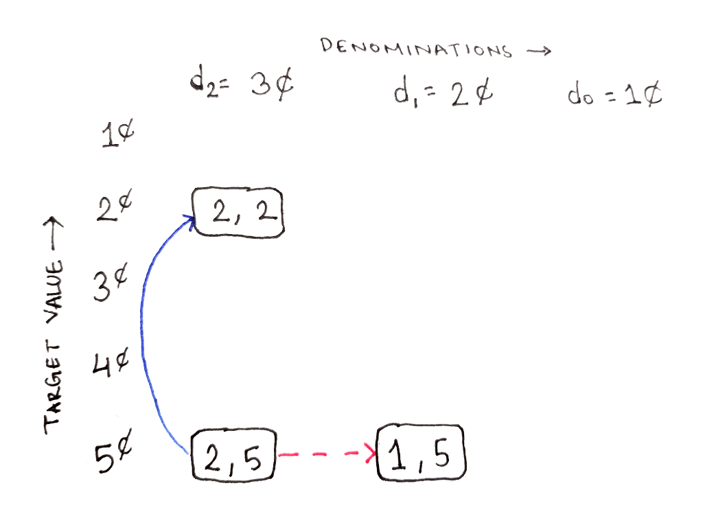
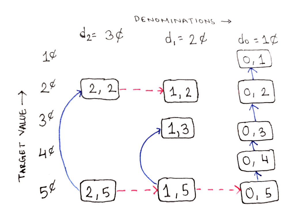
From the subproblem $(1, 5)$, representing the subproblem of reaching 5¢ using only 2¢ and 1¢, we still have both choices available to us. Note that the 1 in the subproblem index corresponds to $d_1$, meaning only $d_1$ and $d_0$ are available to use. This requires us to consider two more subproblems:
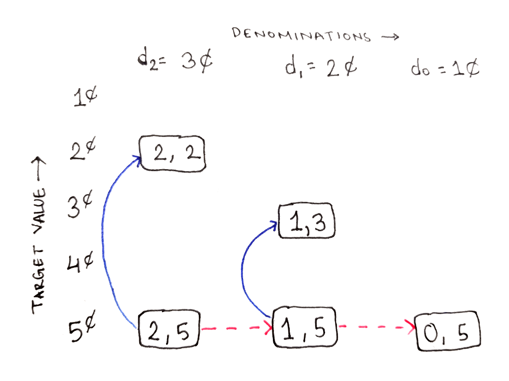
However, from the subproblem $(2, 2)$, representing the subproblem of reaching 2¢ using all three denominations, we cannot use the highest denomination. This is because the highest denomination, 3¢, is greater than the target value of 2¢. So, we only have the option to ignore the highest denomination, moving us one column to the right:
Similarly, from the subproblem $(0, 5)$, representing the subproblem of reaching 5¢ using only 1¢ coins, we have to use the current denomination because there are no other denominations to fall back to. In fact, following the chain of dependencies shows that in this rightmost column, all we can do is go up the column because there is no column to the right:
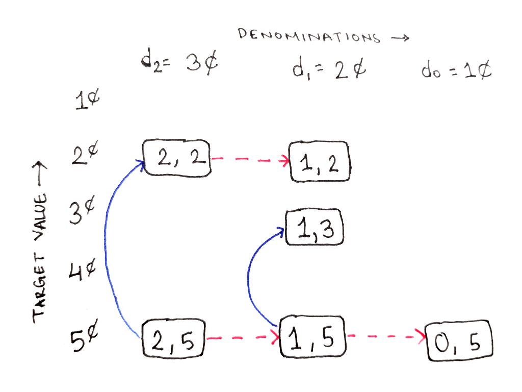
Filling out the rest of the table in this manner reveals the following structure. Any subproblems that are never used are also shown as dimmed cells, and their dependency arrows are not shown.
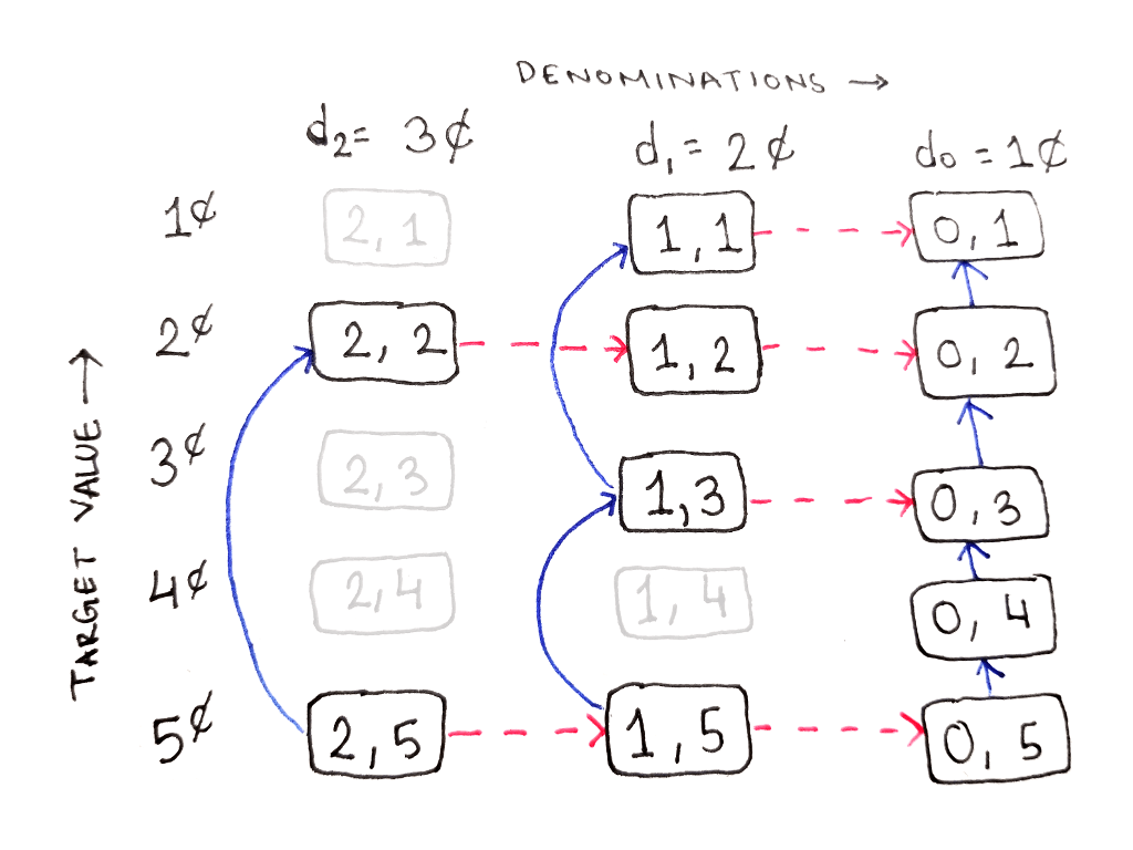
As an exercise, draw out the dependency arrows from the unused subproblems as well. For example, what does the subproblem $(2, 4)$, representing the subproblem of reaching 4¢ using all three denominations, depend on?
Looking at the DAG, we see any cell depends only on cells above it in the same column, and on cells in the column to the right. That means we can compute the subproblems in the following order:
Compute the values one column at a time, starting from the rightmost column.
Within each column, compute the values from the bottom to the top.
Keep around only the values from the previously computed column when computing the next column.
However, notice that not all the values in each column are needed. That means, we don’t strictly need to compute each column fully. Unfortunately, determining which values are needed in each column is not easy to do.
So, while we could implement a bottom-up algorithm, in order to avoid doing more calculations than necessary, we can use memoization instead. When large denominations are present, this can save us a large amount of calculation.
The memoized implementation works mostly like a straightforward translation of the above recurrence relation. The tricky parts is determining when we can’t take a particular choice. We use math.inf as the value for that branch if that branch is not valid. This will cause min() to pick the value of the other branch.
import math

def coins(denominations, target):
    cache = {}

    def subproblem(i, t):
        if (i, t) in cache: return cache[(i, t)]  # memoization

        # Compute the lowest number of coins we need if choosing to take a coin
        # of the current denomination.
        val = denominations[i]
        if val > t: choice_take = math.inf  # current denomination is too large
        elif val == t: choice_take = 1  # target reached
        else: choice_take = 1 + subproblem(i, t - val)  # take and recurse

        # Compute the lowest number of coins we need if not taking any more
        # coins of the current denomination.
        choice_leave = (
            math.inf if i == 0  # not an option if no more denominations
            else subproblem(i - 1, t))  # recurse with remaining denominations

        optimal = min(choice_take, choice_leave)
        cache[(i, t)] = optimal
        return optimal

    return subproblem(len(denominations) - 1, target)
Despite the fact that we used memoization to reduce the number of calculations, that number is still bounded by the total number of subproblems in our graph. Thus, both the run time and space complexity of this algorithm is $O(nc)$, where $n$ is the number of denominations and $c$ is the target value.
To recap, dynamic programming is a technique that allows efficiently solving recursive problems with a highly-overlapping subproblem structure. To apply dynamic programming to such a problem, follow these steps:
Identify the subproblems. Usually, there is a choice at each step, with each choice introducing a dependency on a smaller subproblem.
Write down a recurrence relation.
Determine an ordering for the subproblems. It’s often helpful to draw out the dependency graph, possibly in a single line or a two-dimensional grid.
Implement the recurrence relation by solving the subproblems in order, keeping around only the results that you need at any given point. Alternately, use memoization.
We’ve seen this approach applied to three problems: Fibonacci numbers, the House Robber Problem and the Change Making Problem. This same approach is useful for a wide category of problems, so I encourage you to practice on more problems. If you’d like me to introduce more problems to practice on, along with solutions, let me know!
Thanks to Ty Terdan