
The output of this project. As in all the projects, your output may not look exactly the same, and experimentation is encouraged.
In this project, we will build the foundations of a ray tracer. As a starting point, we will start with a repository with helper functions for writing pixels to an image, then build all the data structures we need for a ray tracer. In the end, you will have an image like the following:
The output of this project. As in all the projects, your output may not look exactly the same, and experimentation is encouraged.
If you are following along with the Javascript and Canvas 2D implementation, clone the repository and check out the commit just prior to the implementation of this project:
git clone https://github.com/avik-das/build-your-own-raytracer-js.git
cd build-your-own-raytracer-js
git checkout before-project-1
If you are using a different reference implementation, use the corresponding repository and check out the same tag. The other implementations are:
https://github.com/avik-das/build-your-own-raytracer-java.gitOne of the fundamental data structures in 3D graphics is the 3D vector. As explained in the refresher on vectors, a 3D vector consists of three coordinates: `x`, `y` and `z`.
Create a representation of a 3D vector with three coordinates. The coordinates will not be integers. Throughout this project and the following ones, you will be adding functionality to this representation.
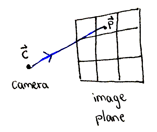
A ray is constructed, originating at the camera and passing through a point on the image plane.
In order to have an image to view, we need an image plane. Represent an image plane in your scene using four vectors: `vec bbx_1`, `vec bbx_2`, `vec bbx_3` and `vec bbx_4`. These are the top-left, top-right, bottom-left and bottom-right corners of the image plane respectively. A good location is:
\begin{array}{rr} \vec{\mathbf{x_1}} & = \langle & 1, & 0.75, & 0 & \rangle \\ \vec{\mathbf{x_2}} & = \langle & -1, & 0.75, & 0 & \rangle \\ \vec{\mathbf{x_3}} & = \langle & 1, & -0.75, & 0 & \rangle \\ \vec{\mathbf{x_4}} & = \langle & -1, & -0.75, & 0 & \rangle \\ \end{array}
You can place the points anywhere you like in the world, but you'll want the image plane to be "flat" and have the same aspect ratio as your image. For example, the reference image above is 256×192, so the image plane should have a width-to-height ratio of 4:3. Exercise: what happens if the image plane has a different aspect ratio, or if it is not flat?
Next, represent a camera as a single vector. Remember that you'll be looking out of the camera toward the image plane, so a good place to put the camera is near the center of the image plane, such as at `vec bbc = (:0, 0, -1:)`. Exercise: what happens if the camea is placed closer or farther from the image plane? What if it's positioned to one side?
Loop through each pixel in the image. Figure out what percentage `alpha` and `beta` along the horizontal and vertical directions it is on the image. For example, if you're looking at the 10th pixel in the horizontal direction, and the width of the image is 100, what is the value of `alpha`?
Using the values of `alpha` and `beta`, perform bilinear interpolation between the corners of the image plane. You'll need to implement the ability to add two vectors, as well as scale a vector by a scalar. Then, you'll need to implement the equations below:
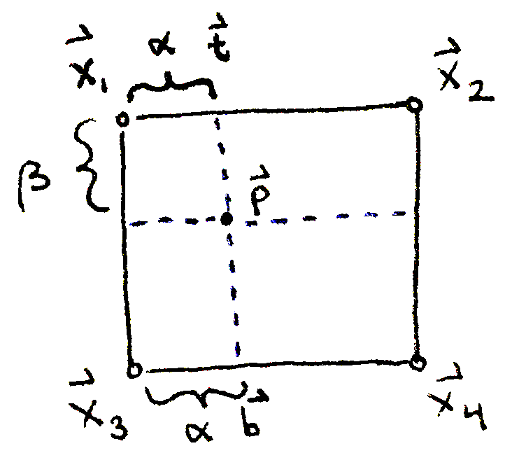
\begin{align} \vec{\mathbf{t}} & = (1 - \alpha) \vec{\mathbf{x}_1} + \alpha \vec{\mathbf{x}_2} \\ \vec{\mathbf{b}} & = (1 - \alpha) \vec{\mathbf{x}_3} + \alpha \vec{\mathbf{x}_4} \\ \vec{\mathbf{p}} & = (1 - \beta) \vec{\mathbf{t}} + \beta \vec{\mathbf{b}} \end{align}
Now that you have a point `vec bbp` on the image plane, create a representation of a ray containing the following two pieces of information:
While this is enough to move onto the next section, we should verify that our rays have been calculated correctly by visualizing the rays. There is a lot of data to visualize, so we'll choose to visualize the direction of each ray. If you used the image plane and camera locations from above, then all of the directions will have the same `z`-coordinate. Exercise: show this is the case. What is the value of the `z`-coordinate?
Figure out what the minimum and maximum values of the `x`- and `y`-coordinates of the ray directions are. Convert the `x`-coordinates into the range `[0, 255]` and use that value as the red component of the color at the corresponding pixel. Do the same for the `y`-coordinate and use it as the value of the green component. Plot these pixels on the image. Exercise: where in the image is the red component the smallest, and where is it the largest? How about the green component? What does this imply for the colors you expect to see at the four corners of the image?
With the locations of the image plane and camera as above, and adding a splash of blue to each pixel, this is the resulting image: