Apr 25, 2019 • Avik Das
In a previous article, I introduced the concept of dynamic programming (DP), and I went over three example problems. In this article, I’ll do a deep-dive into a much harder problem.
I initially wanted to present three problems in order to show as many examples as possible. However, I realized I needed to spend more time explaining my thought process at each step. In this article, I’ll work through only a single problem, emphasizing the visuals that allow me to solve the problem using dynamic programming.
To get the most out of the next example, some linear algebra knowledge is helpful. However, if you’re not familiar with the topic, you’ll need to take the following definitions as givens. (If you want a refresher, Math is Fun goes over matrix multiplication, but you don’t need to know all the details.)
A matrix, for the purposes of this problem, is a two-dimensional array of numbers, with some number of rows and columns. To multiply two matrices together, the number of columns in the first matrix must match the number of rows the second matrix. Suppose the dimensions are $r_1 \times d$ and $d \times c_2$. Then, multiplying these matrices requires $r_1 \times d \times c_2$ operations. The result is a matrix with dimensions $r_1 \times c_2$.
Multiplying matrices is associative, meaning in a chain of multiplied matrices, you can perform the multiplications in any order. Given the following matrices:
The following computations yield the same result, but require different number of operations:
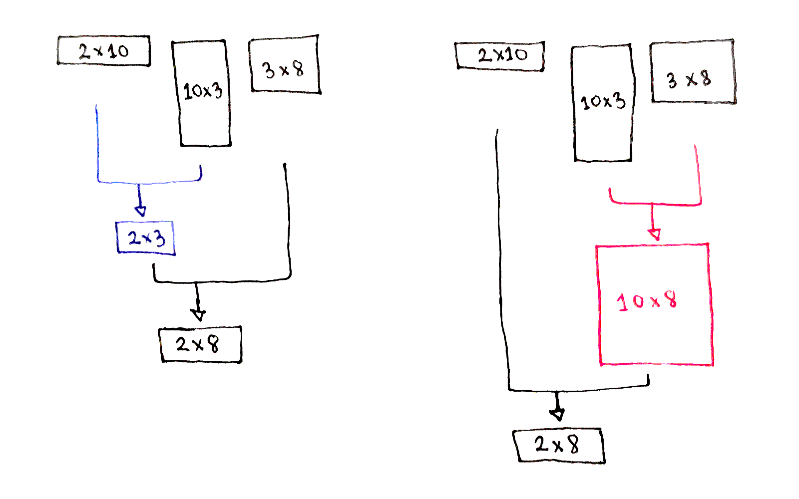
$(AB)C$. The first multiplication generates a $2 \times 3$ matrix, which is then multiplied by $C$. This requires $(2 \times 10 \times 3) + (2 \times 3 \times 8) = 108$ operations.
$A(BC)$. The first multiplication generates a $10 \times 8$ matrix, which is then multiplied by $A$. This requires $(10 \times 3 \times 8) + (2 \times 10 \times 8) = 400$ operations.
It’s much faster to multiply $AB$ first, then multiply the result by $C$.
The Chain Matrix Multiplication Problem asks, given a sequence of matrices, what is the fewest number of operations needed to compute the product of all the matrices? In other words, if we were to parenthesize the given chain of matrix multiplications optimally, how many operations would it take to evaluate that expression?
When breaking down a problem, consider what choices you have. In the Chain Matrix Multiplication Problem, the fundamental choice is which smaller parts of the chain to calculate first, before combining them together.
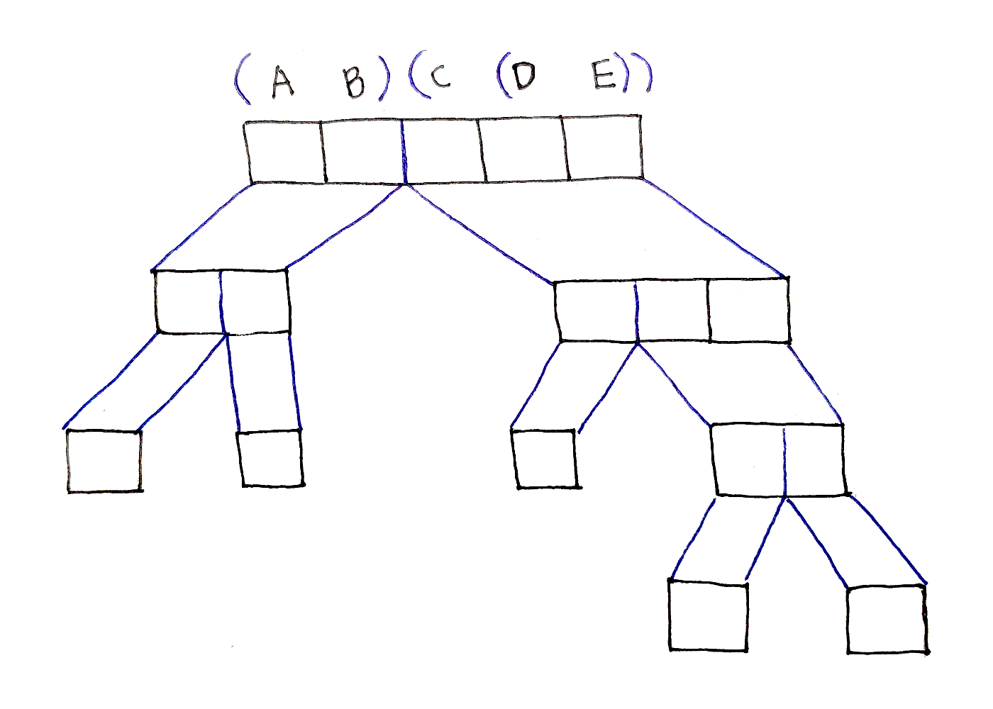
For example, say there are five matrices being multiplied: $ABCDE$. One option is to compute $AB$ and $CDE$ first, then combine the results. Then, to calculate $CDE$, one option is to calculate $DE$ first before multiplying $C$ by the result. This yields the order $(AB)(C(DE))$.
Notice that at each point, we introduced a split, a point in the sequence with left and right subsequences. These subsequences would be multiplied first, yielding two new matrices that can then be multiplied together to form the final result. In this example, we first introduced a split between $B$ and $C$, then a split between $C$ and $D$.
Now, the question is which splits do we choose? Well, the ones that require the fewest operations to compute! To find the best split at each level, we have to try every possible split at that level. In the example above, when deciding where to split $ABCDE$, we have to try four possible splits:
Out of these splits, we pick whichever one requires the fewest operations. The same choice must be made when deciding how to split $CDE$, which requires trying two possible splits.
Is this subproblem structure suitable for a dynamic programming approach? Yes, it is! Firstly, the subproblems are recursive: when finding the optimal split for a sequence, we have to consider the optimal splits for its subsequences. Secondly, the subproblems overlap. In the example above, we have to optimize the subsequence $DE$ when optimizing any sequence ending with $DE$.
Now that we’ve identified the subproblems, we need to formalize that intuition into a recursive function called a recurrence relation. Recall one desired property of this function is it should have integer inputs. This allows ordering the subproblems.
Given our definition of splits above, it sounds like we have a single integer input: the location of the split. But what happens after the split? How do we distinguish between the left and right subsequences?
We actually need to identify not the split point, but the resulting subsequences. That means we want to base our function on two integers $(i,k)$ that correspond to a subsequence starting at index $i$ and ending at index $k$, inclusive. And given that subsequence, we want to know $f(i,k)$, the fewest number of operations needed to multiply the subsequence $(i,k)$. This is convenient because, for a starting sequence of length $n$, the final result we want is $f(0, n-1)$.
First, we need a base case. An easy one is simply the case where there is only one matrix, namely $f(i, i)$ for any $i$ between $0$ and $n-1$. The number of operations needed to multiply a single matrix? Zero, since there’s nothing to multiply!
Next, we need a way to combine subproblems.
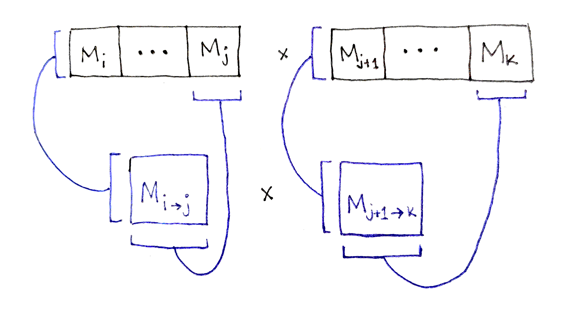
Suppose we’re optimizing a subsequence $(i,k)$. Let’s say we’ve picked a split after index $j$. How many operations does this split require? We can figure that out:
The left subsequence extends from index $i$ to $j$, inclusive. So, it will take $f(i, j)$ operations to calculate the product of that subsequence. The product will be a matrix with the same number of rows as matrix $i$ and the same number of columns as matrix $j$. Call these dimensions $r_i \times c_j$.
The right subsequence extends from index $j+1$ to $k$, inclusive. It will take $f(j+1, k)$ operations to calculate the product. The product will be a matrix with the same number of rows as matrix $j+1$ and the same number of columns as matrix $k$. But, notice that matrix $j+1$ has the same number of rows as the number of columns in matrix $j$. So the product has dimensions $c_j \times c_k$.
Combining the two resulting matrices then takes $r_i \times c_j \times c_k$ operations.
The total number of operations needed to multiply all the matrices in the overall subsequence is the sum of the three factors above. We then minimize this number across all possible split points in the subsequence:
\[\begin{aligned} f(i, i) &= 0 \\ f(i, k) &= \min_{i \leq j < k} \bigg[ f(i, j) + f(j+1, k) + \left( r_i \times c_j \times c_k \right) \bigg] \end{aligned}\]Let’s draw out the directed acyclic graph (DAG) for a problem in which we have five matrices to multiply, $ABCDE$.
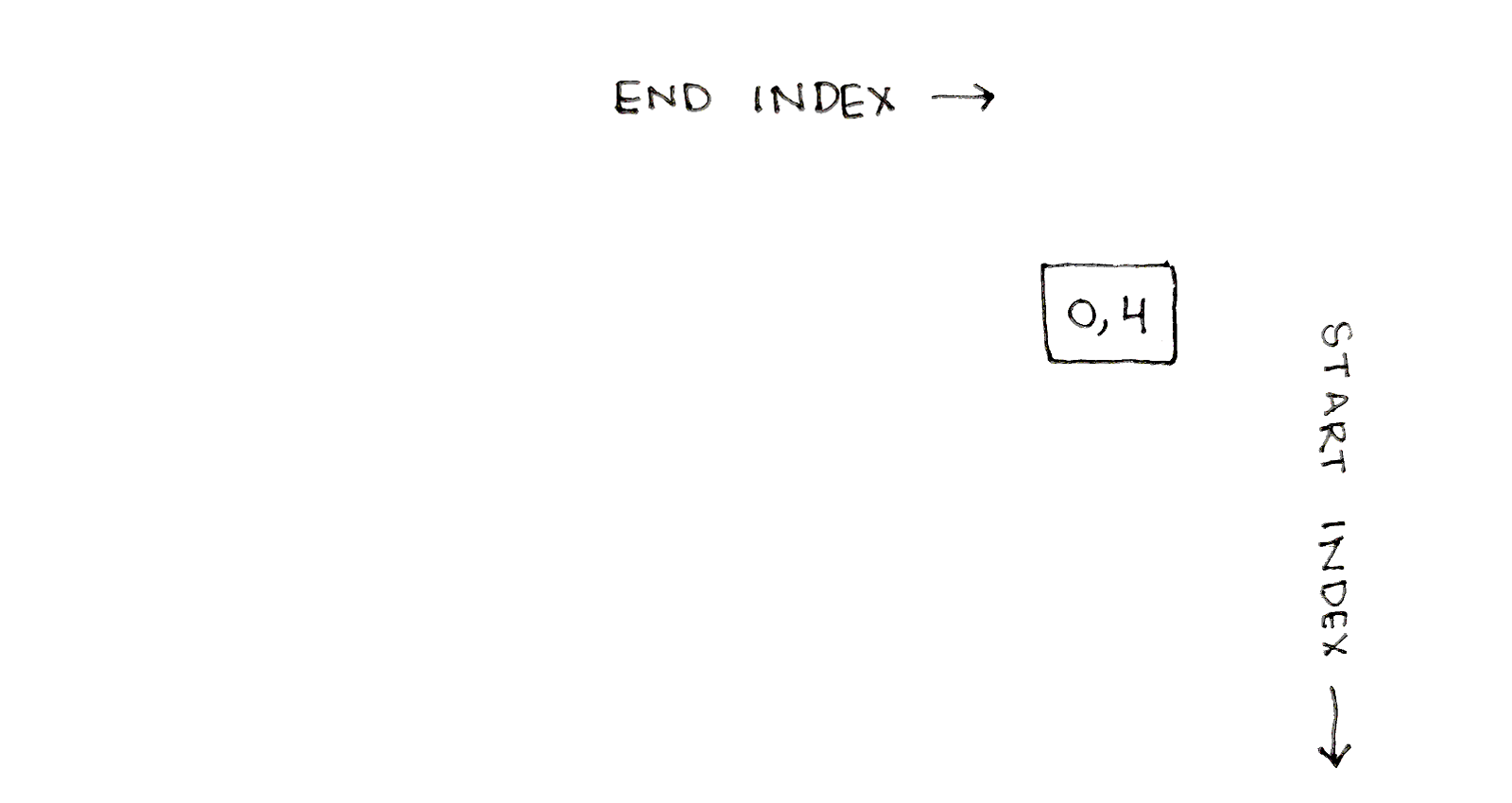
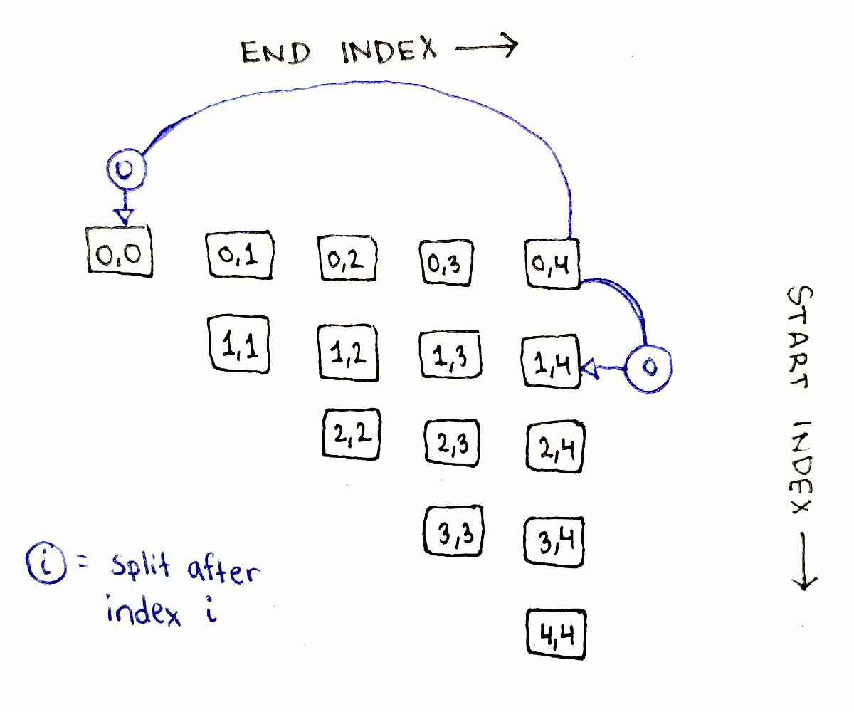
Because our recurrence relation has two integer inputs, we can lay out our subproblems in a two-dimensional table. Recall that each subproblem corresponds to a particular subsequence. Let’s start by putting the end indices on the horizontal axis, increasing from left to right, and the start indices on the vertical axis, increasing from top to bottom. This puts our desired answer at the top right:
The input subsequence needs to be broken down into pairs of subsequences. Let’s start by considering a split after index $1$, meaning breaking down the original sequence into $AB$ and $CDE$. The first subproblem, $(0,1)$, shares the start index with the original sequence, so that subproblem appears in the same row as the original subproblem. Similarly, the second subsequence, $(2,4)$, shares the end index with the original sequence, so that subproblem appears in the same column as the original subproblem.
This pattern of one subproblem appearing in the same row and one subproblem appearing in the same column as the original subproblem will show up consistently.
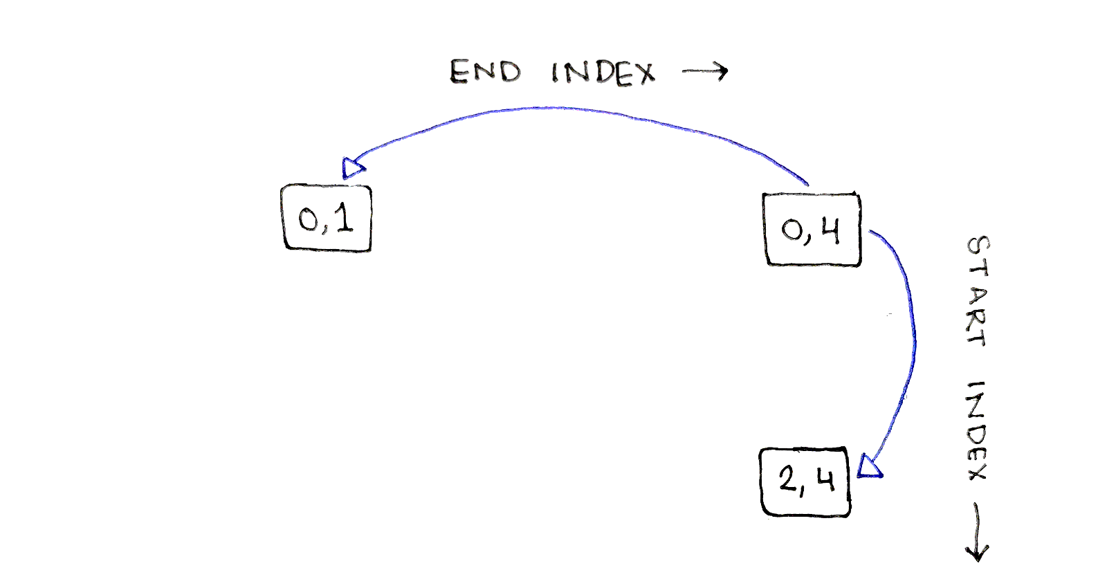
One of these subproblems, $(0,1)$, only has one possible split point, after index $0$. The other subproblem, $(2,4)$, has multiple split points, so let’s split after index $2$. This splits $CDE$ into $C$ and $DE$, resulting in subsequences $(2,2)$ and $(3,4)$:
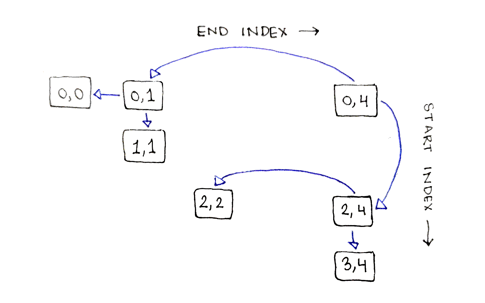
Finally, the subsequence $(3,4)$ has one possible split point, after index $3$, so we end up breaking the corresponding subproblem into subproblems $(3,3)$ and $(4,4)$. At this point, we’ve reached base cases along all our paths, leaving some subproblems untouched.
This particular set of split points corresponds to the order $(AB)(C(DE))$.
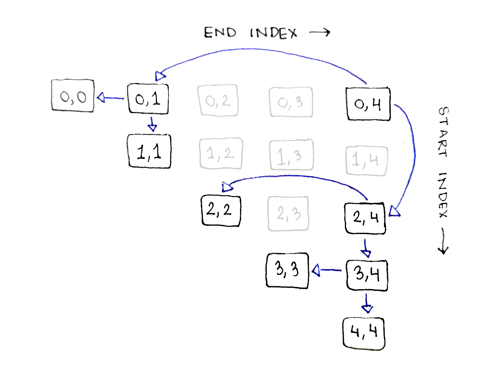
One point to note is only half of the entries in the table are valid subproblems, because it’s required the start index be less than or equal to the end index.
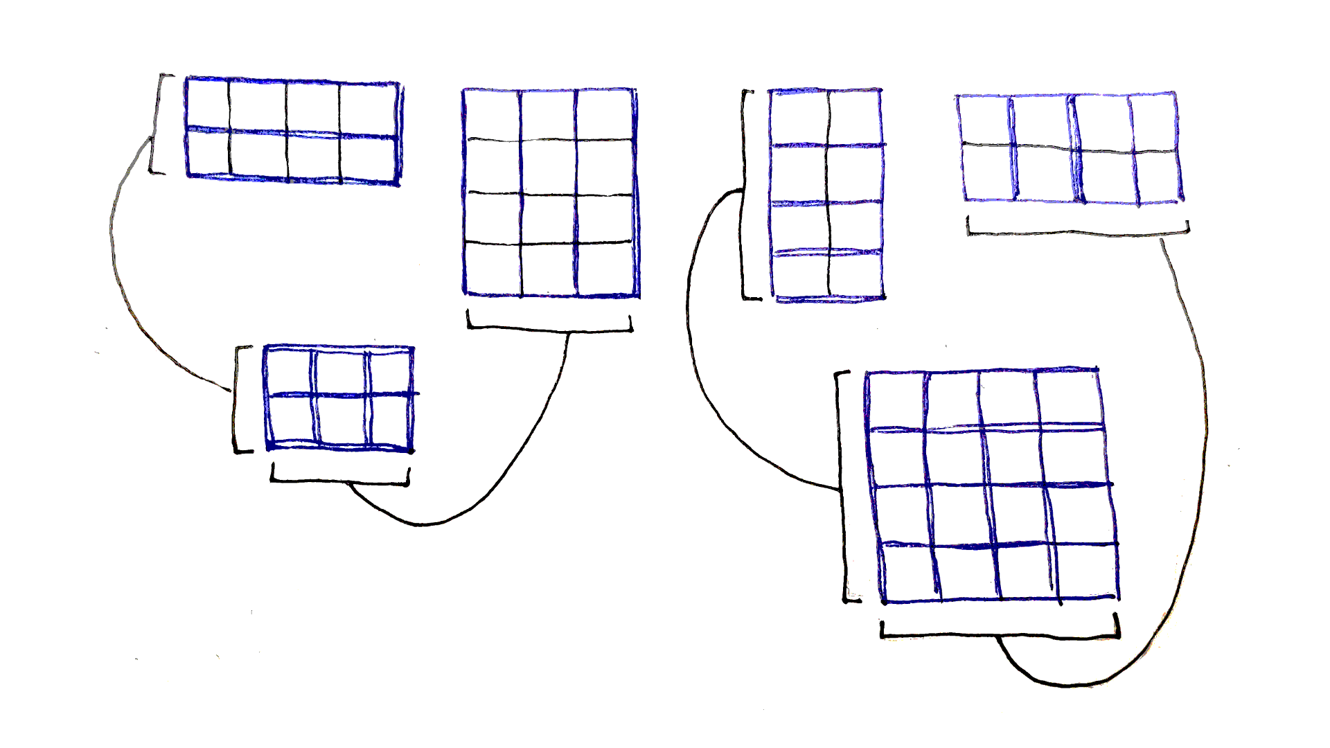
The above dependency graph corresponds to only one choice of split points. We actually need to explore every possible split point. What does this look like? The full dependency graph showing every single connection is a bit too busy to make sense of, but let’s look at all the dependencies for just the biggest subproblem, corresponding to $(0,4)$.
The full sequence has four possible split points, after indices $0$, $1$, $2$, and $3$. For each possible split point $j$, the two subproblems we need to consider are $(0,j)$ and $(j+1,4)$. As we saw earlier, the first of each pair of subproblems will be on the same row as original problem, and the second one will be on the same column. With that knowledge, we can enumerate each pair of dependencies:
The pattern is exactly the same for all the subproblems: go down all the entries in the same row and column as the subproblem.
With such a deep analysis of the dependency graph, we have a really good idea of how to approach an implementation. The only remaining part is defining an order in which to solve the subproblems. Intuitively, it seems we should go along the left-most diagonal of the dependency graph, as those cells have no dependency. But what does that diagonal correspond to?
This is where the visual structure of the dependency graph really shines. Let’s rotate the graph so the left-most diagonal is now at the bottom:
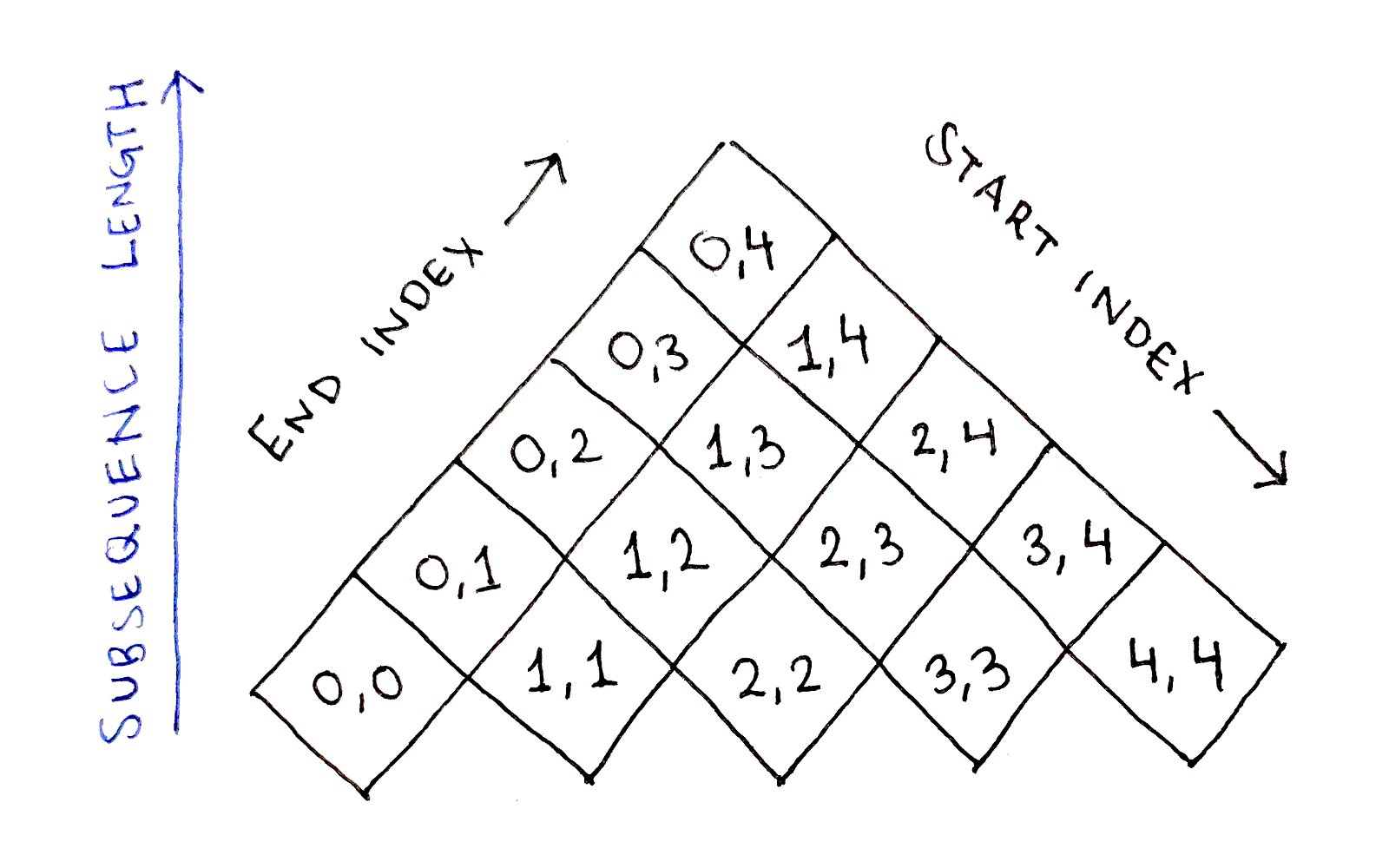
Now, it’s clear the cells in each row have the same difference between their start and end indices. Thus, the bottom row corresponds to subsequences of length $1$, followed by subsequences of length $2$ in the row above, and so on. This intuition also makes it clear any cell depends only on cells in lower rows, which makes sense since subsequences can only depend on shorter subsequences. Even more strictly, no row depends on itself either.
This gives us a natural order in which to proceed:
Proceed in increasing order of subsequence length, from $1$ to $n$ inclusive. Call this length $l$.
Solve all subproblems corresponding to subsequences of length $l$, in any order. An easy option is to proceed in increasing order of start index, from $0$ to $n - l$ inclusive.
The only remaining aspect is how to represent the input. For simplicity, we will specify a list of pairs, with each pair representing the number of rows and columns for the corresponding matrix in the original sequence.
In Python:
def chain_matrix(matrices):
    # Ideally do error checking to make sure the columns of each matrix match
    # the rows of the next matrix.

    def cols(i): return matrices[i][1]
    def rows(i): return matrices[i][0]

    n = len(matrices)
    f = {}  # cached values of the recurrence relation

    for l in range(1, n + 1):
        for start in range(0, n - l + 1):
            # Base case
            if l == 1:
                f[(start, start)] = 0
                continue

            # Recursive case
            end = start + l - 1
            f[(start, end)] = min(
                f[(start, mid)] +
                f[(mid + 1, end)] +
                rows(start) * cols(mid) * cols(end)
                for mid in range(start, end)  # end is exclusive
            )

    return f[(0, n - 1)]
Try it with the original example presented at the beginning of the article:
print(chain_matrix([(2, 10), (10, 3), (3, 8)]))
Suppose the input sequence has $n$ matrices.
The dependency graph is an $n \times n$ table, and about half of the cells correspond to valid subproblems. Thus, there are approximately $\frac{n^2}{2}$ subproblems in the dependency graph, meaning on the order of $O(n^2)$ subproblems to calculate. Unfortunately, we can’t throw away intermediate values because of how later subproblems depend on many earlier subproblems. This means the space complexity is $O(n^2)$.
To compute a subproblem, we have to look at all the “smaller” subproblems in the same row and same column in the table. That means, we might have to do as many as $O(n)$ calculations to put the smaller subproblems together into a single bigger subproblem. This applies to all $O(n^2)$ subproblems, so the final time complexity is $O(n^3)$. Not great, but at least it’s not exponential!
The Chain Matrix Multiplication Problem is an example of a non-trivial dynamic programming problem. When applying the framework I laid out in my last article, we needed deep understanding of the problem and we needed to do a deep analysis of the dependency graph:
We identified the subproblems as breaking up the original sequence into multiple subsequences.
We formulated a recurrence relation by analyzing how subproblems combined to form larger results.
We determined an ordering for the subproblems by visualizing the dependency graph as a two-dimensional table from multiple angles.
Finally, we implemented the recurrence relation by solving the subproblems in order.
While this problem illustrate the principles of dynamic programming, I haven’t found solid real-world applications of the problem. If anyone knows any applications, I would be interested to hear them. In a later article, however, I will cover a more practical application of dynamic programming, so stay tuned!