
An overhead view of a surfer prominently visible in the middle of a calm ocean, with turbulent waves behind them on the right. Credit goes to Kiril Dobrev on Pixabay.
May 14, 2019 • Avik Das
Dynamic programming has a reputation as a technique you learn in school, then only use to pass interviews at software companies. Indeed, most developers do not regularly work on problems where dynamic programming is needed. Ultimately, dynamic programming is a technique for efficiently solving problems that can be broken down into highly-repeated subproblems, and as a result, is useful in many situations.
In this article, I’ll work through an interesting real-world application of dynamic programming: seam carving. The problem and proposed technique is discussed in detail in the paper Seam Carving for Content-Aware Image Resizing by Avidan and Shamir. (The paper is freely available if you search for the title.)
This article is part of an ongoing series on dynamic programming. If you need a refresher on the technique, see my graphical introduction to dynamic programming.
In order to solve a real-world problem with dynamic programming, it’s necessary to frame the problem in a way where dynamic programming is applicable. This section covers the necessary setup for our chosen problem.
The authors of the original paper introduce content-aware image resizing, that is changing the width or height of an image in a way that intelligently accounts for the contents of that image. I’ll let the paper go into details, but here’s a brief overview. Suppose you want to resize the following image of a surfer:

An overhead view of a surfer prominently visible in the middle of a calm ocean, with turbulent waves behind them on the right. Credit goes to Kiril Dobrev on Pixabay.
As the paper discusses in detail, there are multiple ways to reduce the width of the image. Cropping and scaling come to mind, with their associated downsides, but there’s also the possibility of removing columns of pixels from the middle of the image. As you might imagine, doing so leaves a visible line in the image where the image on the left and right don’t match up. And even after doing all this, there’s only so much of the image that can be removed this way.

What Avidan and Shamir show in their paper is a technique known as seam carving. The technique first identifies “low-energy” areas of the image that are less interesting, then finds the lowest-energy “seams” that weave through the image. In the case of reducing the width of an image, seam carving finds a vertical seam that stretches from the top of the image to the bottom, moving left or right by at most one pixel from one row to the next.
In the surfer image, the lowest-energy seam goes through the middle of the image, where the water is the calmest. This matches our intuition.

By identifying the lowest-energy seam, then removing it, we reduce the width of the image by one pixel. Repeating this process again and again lets us reduce the width of the image substantially.

Again, following our intuition, the algorithm has removed the still water in the middle, as well as the water on the left of the image. Unlike the crop, however, the texture of the water on the left is preserved, and there are no jarring transitions. It’s true that there are some less than perfect transitions in the middle of the image, but for the most part, the result looks natural.
The magic is in finding the lowest-energy seam. To do so, we first assign each pixel of the image an energy. Then, we apply dynamic programming to find the lowest-energy path through the image, an algorithm we’ll discuss in detail in the next section. First, let’s cover how energy values are assigned to the pixels of the image.
The paper discusses a few different energy functions and the effect they have on resizing. We’ll keep it simple with an energy function that simply captures how sharply the color in the image changes around each pixel. For the sake of completeness, I’ll describe the energy function in a little bit of detail in case you want to implement it yourself, but this part of the computation is simply setup for the dynamic programming later.

To compute the energy of a single pixel, we look at the pixels to the left and right of that pixel. We find the squared component-wise distance between them, that is compute the squared difference between the red components, the squared difference between the green components and the squared difference between blue components, then add them up. We do the same for the pixels above and below the center pixel. Finally, we add up the horizontal and vertical distances.
\[\begin{aligned} | \Delta x |^2 &= (\Delta r_x)^2 + (\Delta g_x)^2 + (\Delta b_x)^2 \\ | \Delta y |^2 &= (\Delta r_y)^2 + (\Delta g_y)^2 + (\Delta b_y)^2 \\ \end{aligned}\] \[\begin{aligned} e(x, y) &= | \Delta x | ^2 + | \Delta y | ^2 \end{aligned}\]The only caveat is if a pixel is up against, say, the left edge, there is no pixel to the left. In that case, we just compare the pixel itself to the pixel to the right. A similar adjustment is made for pixels on the top, right and bottom edges.
This energy function is large when the surrounding pixels are very different in color, and small when the surrounding pixels are similar.

This energy function works well for the surfer image. However, the energy function takes on a very large range of values, so when visualizing the energy, it looks like most of the image has zero energy. In reality, those regions simply have low energy values compared to the highest-energy regions. To make the energy function easier to visualize, I’ve zoomed in on the surfer and brightened up the region.
With the energy computed for each pixel, we can now look for the lowest-energy seam that goes from the top of the image down to the bottom. The same analysis applies for horizontal seams going from the left edge to the right edge, which would allow us to reduce the height of the original image. However, we’ll focus on vertical seams.
Let’s start by defining the lowest-energy seam:
A seam is sequence of pixels, exactly one per row. The requirement is that between two consecutive rows, the $x$ coordinate can only vary by at most one. This keeps the seam connected.
The lowest-energy seam is the one whose total energy across all the pixels in the seam is minimized.
It’s important to notice the lowest-energy seam may not pass through all the lowest-energy pixels in the image. It’s the total energy of the seam being minimized, not the individual pixel energies.
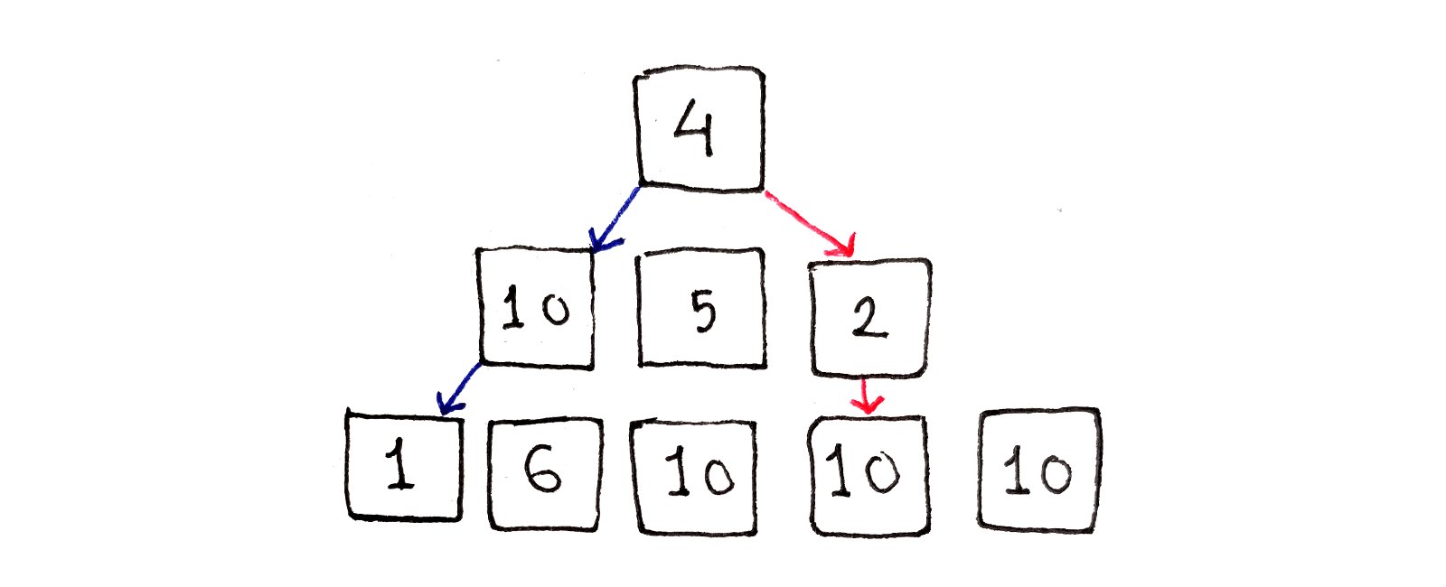
We can see starting at the top row and trying to pick the lowest-energy pixel in the next row doesn’t work. By going to the pixel with an energy of $2$, we are forced into a high-energy region of the image. Instead, if we had chosen to go with the higher-energy pixel at the left side of the middle row, we would have access to the lower-energy region at the bottom left.
The problem with the greedy approach above is that, when deciding how to continue a seam, we don’t take into account the rest of the seam yet to come. We can’t look into the future, but we can capture everything we know up to this point in order to look at the past.
Let’s turn our choice on its head. Instead of choosing between multiple pixels to continue a single seam, let’s choose between multiple seams to connect to a single pixel. What we’ll do is look at each pixel and choose between the pixels in the above row we can connect with. If each of the pixels in the above row encodes the path taken up to that point, we essentially look at the full history up to that point.
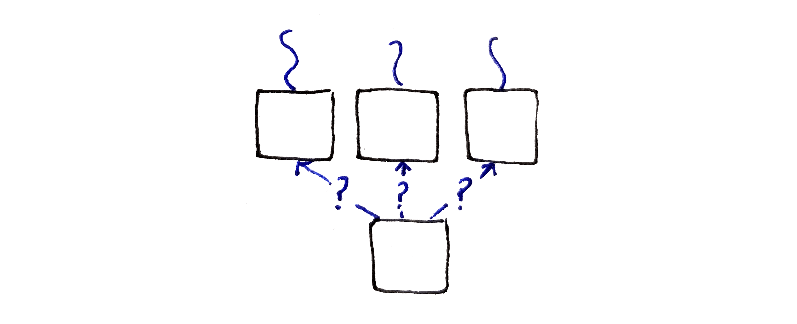
This suggests having a subproblem corresponding to each pixel in the image. Because the subproblem needs to capture the best path up to that pixel, a good choice is associating with each pixel the energy of the lowest-energy seam ending at that pixel.
Unlike the greedy approach, the above approach essentially tries all possible paths through the image. It’s just that, when trying all possible paths, the same subproblems are solved again and again, making this approach a perfect candidate for dynamic programming.
As usual, we now have to formalize the above intuition into a recurrence relation. There is a subproblem corresponding to each pixel in the original image, so the inputs to our recurrence relation can just be the $x$ and $y$ coordinates of that pixel. This gives us integer inputs, allowing easy ordering of subproblems, as well as the ability to store previously-computed values in a two-dimension array.
We’ll define a function $M(x, y)$ that represents the energy of the lowest-energy vertical seam that starts at the top of the image and ends at pixel $(x, y)$. The name $M$ was chosen because that’s what the paper defines.
First, we need a base case. In the top row of the image, all the seams ending at those pixels are just one pixel long, because there are no pixels farther above. So, the energy of the lowest-energy seam ending at those pixels are just the energies of those pixels:
\[\begin{aligned} M(x, 0) &= e(x, 0) \\ \end{aligned}\]For all the remaining pixels, we have to look at the pixels in the row directly above. Because a seam has to be connected, we only look at the pixels directly to the top-left, directly above and directly to the top-right. From those pixels, we’ll pick the lowest-energy seam ending at one of those pixels, and add on the current pixel’s energy:
\[\begin{aligned} M(x, y) &= e(x, y) + \min \begin{cases} M(x - 1, y - 1) \\ M(x, y - 1) \\ M(x + 1, y - 1) \end{cases} \end{aligned}\]As an edge case, we need to consider what happens when the pixel we’re looking at is along the left or right edge of the image. In these cases, we omit either $M(x - 1, y - 1)$ for pixels on the left edge or $M(x + 1, y - 1)$ for pixels on the right edge.
Finally, we need to extract the energy of the lowest energy seam that spans the entire height of the image. This means looking at the bottom row of the image and picking the lowest energy seam ending at one of those pixels. Assuming the image is $W$ pixels wide and $H$ pixels tall, we want:
\[\min_{0 \le x < W} M(x, H - 1)\]With this definition, we have a recurrence relation with all the properties we want:
Because each subproblem $M(x, y)$ corresponds to a single pixel in the original image, the subproblem dependency graph is really easy to visualize. Just lay out the subproblems in a two-dimensional grid, just like in the original image!
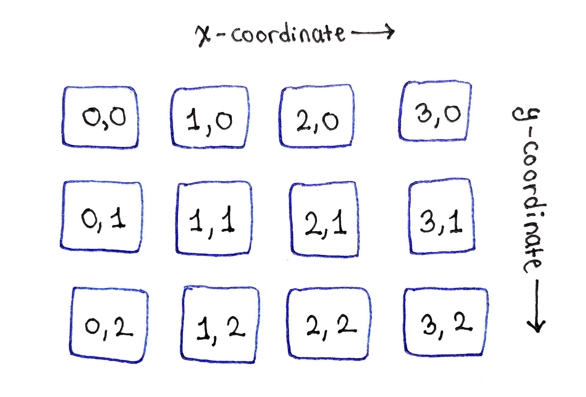
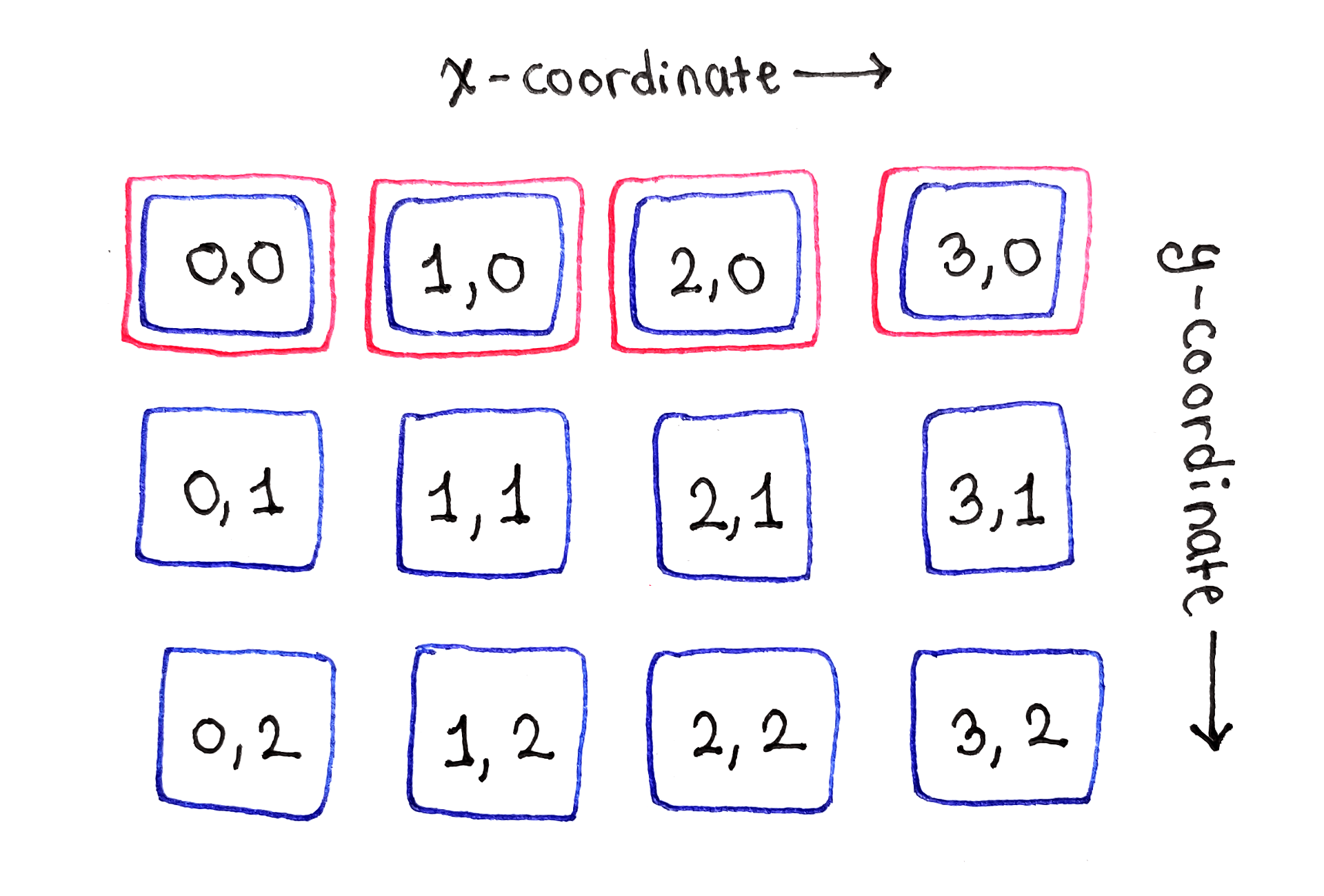
As the base case for the recurrence relation shows, the top row of subproblems, corresponding to the top row of the image, can simply be initialized with the individual energy values for those pixels.
The second row is where the dependencies start appearing. First, on the left-most cell in the second row, we encounter a literal edge case. Because there are no cells to left, the cell marked $(1, 0)$ depends only on the cells directly above and to the top-right of it. The same will happen later with the left-most cell in the third row.
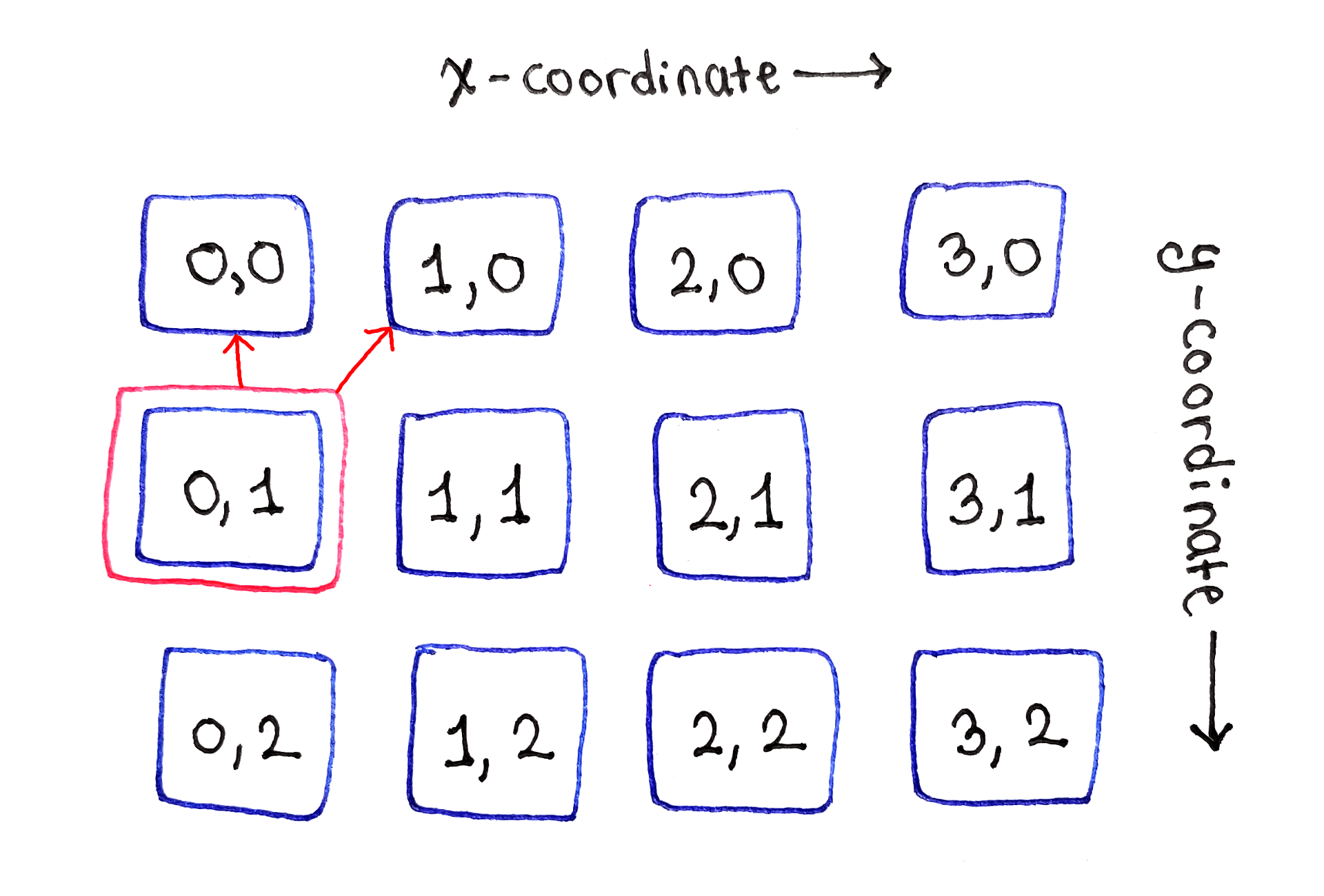
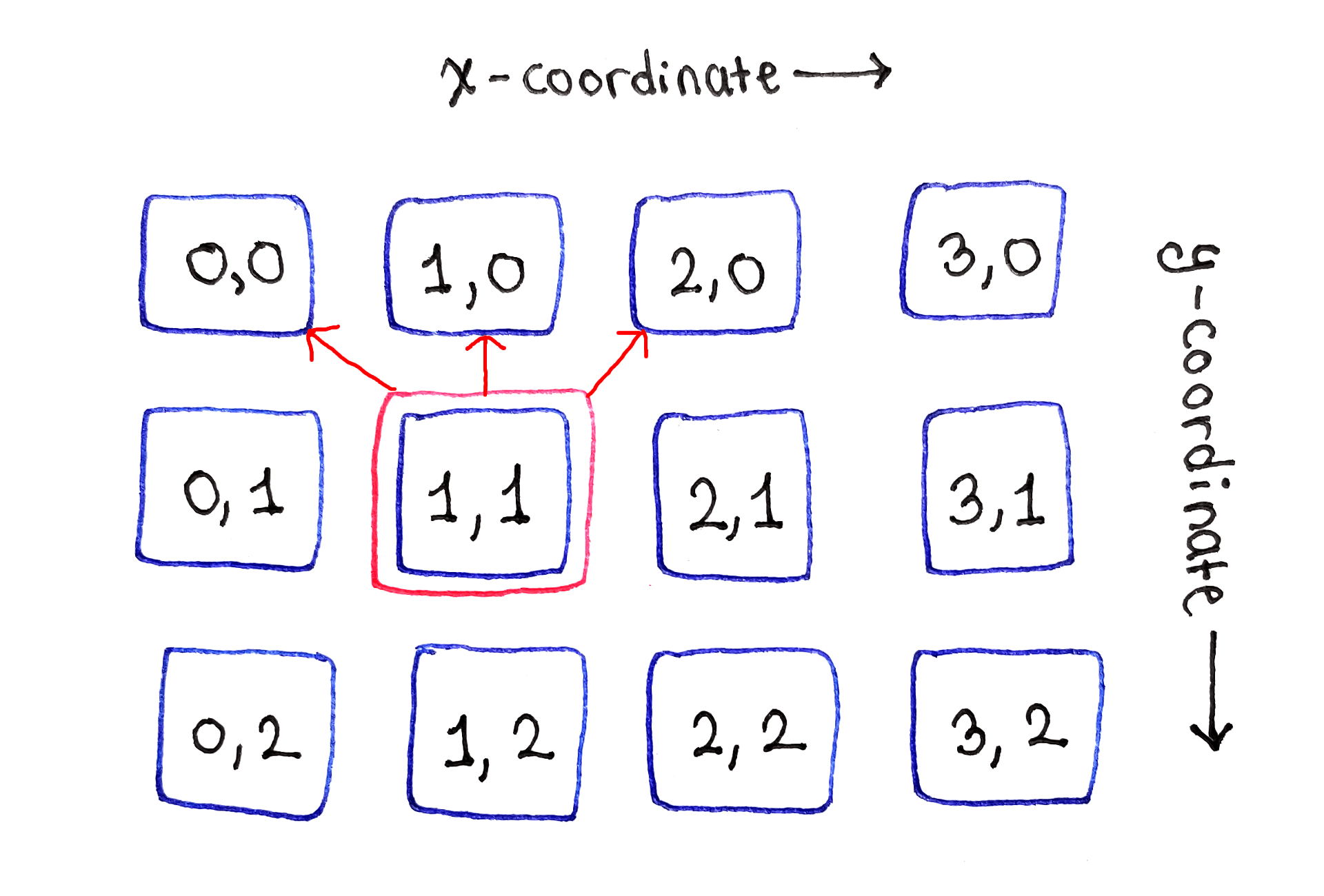
Moving onto the second cell in the second row, labeled $(1, 1)$, we see the most typical manifestation of the recurrence relation. That cell depends on the cells to the top-left, directly above and to the top-right of it. This dependency structure applies to all “middle” cells in the second and subsequent rows.
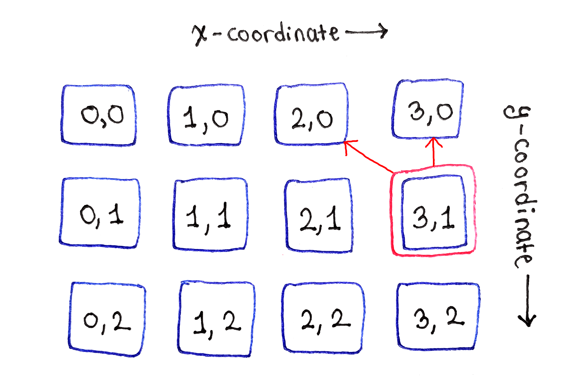
Finally, the right edge presents the second edge case. Because there are no more cells to the right, this cell depends only on the cells directly above and to the top-left.
Finally, this process is repeated for all subsequent rows.
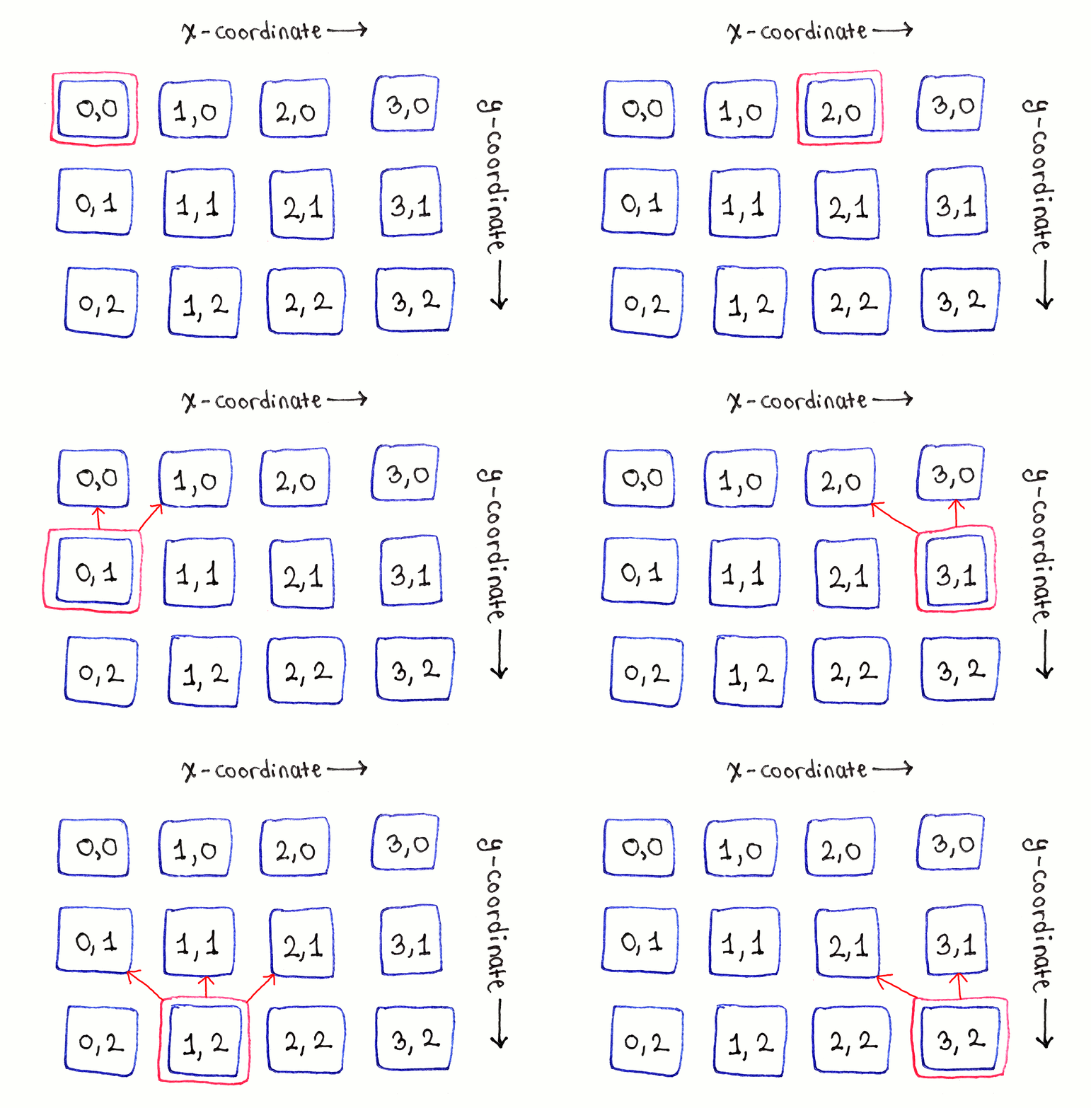
While the full dependency graph is intimidating due to the sheer number of arrows, looking at each subproblem one by one helps establish noticeable patterns.
From the above analysis, we have an ordering we can exploit:
Because each row only depends on the previous one, we only need to keep two rows of data available: one for the previous row, and one for the current row. In fact, by going from left to right, we can actually throw away individual elements from the previous row as they are used up. However, this complicates the algorithm, as we have to figure out which parts of the previous row can be discarded and how to discard them.
In the following Python code, the input is a list of rows, where each row is a list of numbers representing individual pixel energies for the pixels in that row. The input is named pixel_energies, and pixel_energies[y][x] represents the energy of the pixel at coordinates $(x, y)$.
Start by computing the seam energies of the top row by simply copying over the individual pixel energies at the top row:
previous_seam_energies_row = list(pixel_energies[0])
Next, loop through the remaining rows of the input, computing the seam energies for each row. The trickiest part is determining which elements of the previous row to reference, since there are no pixels to the left of the left edge or to the right of the right edge.
In each iteration, a new list of seam energies is created for the current row. At the end of the iteration, replace the previous row’s data with the current row’s data for the next iteration. This is how we throw away the previous row.
# Skip the first row in the following loop.
for y in range(1, len(pixel_energies)):
    pixel_energies_row = pixel_energies[y]

    seam_energies_row = []
    for x, pixel_energy in enumerate(pixel_energies_row):
        # Determine the range of x values to iterate over in the previous
        # row. The range depends on if the current pixel is in the middle of
        # the image, or on one of the edges.
        x_left = max(x - 1, 0)
        x_right = min(x + 1, len(pixel_energies_row) - 1)
        x_range = range(x_left, x_right + 1)

        min_seam_energy = pixel_energy + \
            min(previous_seam_energies_row[x_i] for x_i in x_range)
        seam_energies_row.append(min_seam_energy)

    previous_seam_energies_row = seam_energies_row
Finally, at the end, previous_seam_energies_row contains the seam energies for the bottom row. Find the minimal value in this list, and that’s the answer!
min(seam_energy for seam_energy in previous_seam_energies_row)
You can test this implementation by wrapping the above code in a function, then calling the function with a two-dimensional array you construct. The following input data has been constructed so that a greedy approach would fail, but also so that there is an obvious lowest-energy seam:
ENERGIES = [
    [9, 9, 0, 9, 9],
    [9, 1, 9, 8, 9],
    [9, 9, 9, 9, 0],
    [9, 9, 9, 0, 9],
]

print(min_seam_energy(ENERGIES))
There is one subproblem corresponding to each pixel in the original image. For each subproblems, there are at most $3$ dependencies, so we do a constant amount of work to solve each subproblem. Finally, we go through the last row one more time. Thus, if the image is $W$ pixels wide and $H$ pixels tall, the time complexity is $O(W \times H + W)$.
At each time, we store two lists, one for the previous row and one for the current row. The first one has $W$ elements, and second one grows to have $W$ elements at most. Thus, the space complexity is $O(2W)$, which is simply $O(W)$.
Note that if we actually discarded elements from the previous row’s data, we would shrink the previous row’s list at about the same rate as the current row’s list. Thus, the space complexity would still be $O(W)$. Depending on the width of the image, the constant factor can certainly matter, but usually, it’s not a big deal.
Now that we’ve found the energy of the lowest-energy vertical seam, what do we do with this information? It turns out we don’t actually care about the energy of the seam, but the seam itself! The problem is, from the ending position of the seam, we don’t have a way to back track through the rest of the seam.
This is something I’ve skipped over in previous articles, but the same concern applies to many dynamic programming problems. For example, if you remember the House Robber Problem, we found a numerical value corresponding to the maximum value we could extract, but not which houses yielded that total value.
The answer is a common one: store back pointers. In the seam carving problem, we don’t just want the value of the seam energy at each pixel. We also want to know which of the pixels in the previous row led to that energy. By storing this information, we can follow these pointers all the way to the top of the image, yielding the pixels that make up the lowest-energy seam.
First, let’s create a class to store both the energy and the back pointers. The energy will be used for the calculation of subproblems. Since the back pointer simply identifies which pixel in the previous row yielded the current energy, we can represent the pointer as just the x coordinate.
class SeamEnergyWithBackPointer():
    def __init__(self, energy, x_coordinate_in_previous_row=None):
        self.energy = energy
        self.x_coordinate_in_previous_row = x_coordinate_in_previous_row
The result of each subproblem will be an instance of this class, instead of just a number.
At the end, we’ll need to back track through the entire height of the image, following back pointers, to reconstruct the lowest-energy seam. This unfortunately means we need to keep back pointers around for all the pixels in the image, not just for the previous row.
To achieve this, we will just keep around the full result of all subproblems, though we could technically discard the numerical seam energies of earlier rows. We can store these results in a two-dimensional array that looks just like the input array.
Let’s start with the first row, which just contains the individual pixel energies. Because there is no previous row, all the back pointers are None, but for consistency, we’ll store instances of SeamEnergyWithBackPointers anyway:
seam_energies = []

# Initialize the top row of seam energies by copying over the top row of
# the pixel energies. There are no back pointers in the top row.
seam_energies.append([
    SeamEnergyWithBackPointer(pixel_energy)
    for pixel_energy in pixel_energies[0]
])
The main loop works mostly the same as the previous implementation, with the following differences:
The data for the previous row contains instances of SeamEnergyWithBackPointer, so when calculating the value of the recurrence relation, we have to look inside those objects for the seam energy.
When storing the data for the current pixel, we have to construct a new instance of SeamEnergyWithBackPointer. This is where we’ll store the seam energy for the current pixel, but also the x coordinate from the previous row used to calculate the current seam energy.
At the end of each row, instead of discarding the previous row’s data, we simply append the current row’s data to seam_energies.
# Skip the first row in the following loop.
for y in range(1, len(pixel_energies)):
    pixel_energies_row = pixel_energies[y]

    seam_energies_row = []
    for x, pixel_energy in enumerate(pixel_energies_row):
        # Determine the range of x values to iterate over in the previous
        # row. The range depends on if the current pixel is in the middle of
        # the image, or on one of the edges.
        x_left = max(x - 1, 0)
        x_right = min(x + 1, len(pixel_energies_row) - 1)
        x_range = range(x_left, x_right + 1)

        min_parent_x = min(
            x_range,
            key=lambda x_i: seam_energies[y - 1][x_i].energy
        )

        min_seam_energy = SeamEnergyWithBackPointer(
            pixel_energy + seam_energies[y - 1][min_parent_x].energy,
            min_parent_x
        )

        seam_energies_row.append(min_seam_energy)

    seam_energies.append(seam_energies_row)
With the entire subproblem table filled out, we can now reconstruct the lowest-energy seam. Start by finding the x coordinate in the bottom row that corresponds to the lowest-energy seam:
# Find the x coordinate with minimal seam energy in the bottom row.
min_seam_end_x = min(
    range(len(seam_energies[-1])),
    key=lambda x: seam_energies[-1][x].energy
)
Now, proceed from the bottom of the image up to the top, varying $y$ from len(seam_energies) - 1 down to 0. In each iteration, add the current ($x, y)$ pair to a list representing our seam, then set the $x$ value to whatever the SeamEnergyWithBackPointer object in the current row points to.
# Follow the back pointers to form a list of coordinates that form the
# lowest-energy seam.
seam = []
seam_point_x = min_seam_end_x
for y in range(len(seam_energies) - 1, -1, -1):
    seam.append((seam_point_x, y))

    seam_point_x = \
        seam_energies[y][seam_point_x].x_coordinate_in_previous_row

seam.reverse()
This builds up the seam from bottom to top, so reverse the list if you want the coordinates from top to bottom.
The time complexity is similar to before, because we still need to process each pixel once. At the end, in addition to looking at the last row for the lowest seam energy, we then go up the entire height of the image to reconstruct the seam. Thus, for a $W \times H$ image, the time complexity is $O(W \times H + W + H)$.
As for space, we still store a constant amount of data for each subproblem, but now we don’t discard any of the data. Thus, we use $O(W \times H)$ space.
Once the lowest-energy vertical seam has been found, we can simply copy over the pixels from the original image into a new one. Each row of the new image has all the pixels from the corresponding row of the original image, except for the pixel from the lowest-energy seam. Because we remove a single pixel in each row, starting with a $W \times H$ image, we end up with a $(W - 1) \times H$ image.
We can repeat this process by recomputing the energy function on the new image, then finding the lowest-energy seam in the new image. It seems tempting to find more than one low-energy seam in the original image, then remove them all in one go. The problem is that two seams may cross each other, sharing a pixel in the middle. When the first of these two seams is removed, the second seam is no longer valid because it’s missing a pixel.
The above video shows the seam removal process applied to the surfer image. I made the video by taking the image at each iteration, and overlaying a visualization of the lowest-energy seam at that iteration.
That was a lot of in-depth explanation, so let’s finish off with some more pretty pictures! Take the following photo of a rock formation in Arches National Park:

A rock formation with a hole in the middle in Arches Nation Park. Credit goes to Mike Goad on Flickr.
The energy function for this image:

This yields the following lowest-energy seam. Notice the seam goes through the rock on the right, entering the rock formation right where the lit part on the top of the rock matches up with the color of the sky. Perhaps we should choose a better energy function!

Finally, after resizing the arch image:

The result is definitely not perfect, with many of the edges in the original image distorted in the resized image. One improvement may be to implement one of the other energy functions discussed in the paper.
Dynamic programming, while typically encountered in academic settings, is a useful technique for solving complex problems. In this article, we covered one application of dynamic programming: content-aware image resizing using seam carving.
We applied the same principles of breaking down the problem into smaller subproblems, analyzing the dependencies between these subproblems, then solving the subproblems in an order that minimizes the space and time complexities of the algorithm. Additional, we also explored the use of back pointers to not only find the minimized numerical value we computed, but the specific choices that yielded that value. These pieces were then applied to a real-world problem, which requires both pre- and post-processing to make the dynamic programming algorithm actually useful.