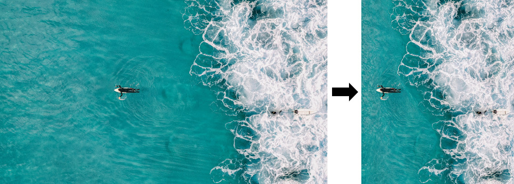
An overhead view of a surfer in the middle of a calm ocean, with the resized result on the right. Credit for original image goes to Kiril Dobrev on Pixabay.
Jul 29, 2019 • Avik Das
One observation I pointed out in my post about content-aware image resizing was that the energy function used to define “interesting” areas of an image affects the result of the resizing. In this post, I’ll explore how we can refine our use of the energy function for even better results than we’ve seen so far.
I won’t go into all the details from my last post, but I’ll recap the most important points. In content-aware image resizing, the goal is to remove pixels from an image in a way that minimizes visual artifacts, like stretching or sharp, unnatural boundaries.
One way to do this is to assign to each pixel in the source image an “energy” depending on how much the surrounding pixels change color. This approach approximates identifying interesting areas of the images. Next, dynamic programming is used to find the lowest-energy “seam” in the image. A seam is a connected sequence of pixels spanning the height of an image, with one pixel per row. These pixels can then be removed, leaving behind a smaller image with barely any effect on the visual coherence of the image.
In my previous post, one example I showed was the following image of a surfer in the middle of the ocean. By removing successive seams, it was possible to remove the less visually interesting still water. You can see an animation of the resizing happening over time.
An overhead view of a surfer in the middle of a calm ocean, with the resized result on the right. Credit for original image goes to Kiril Dobrev on Pixabay.
The exact algorithm is detailed, with example code, in my previous post.
Unfortunately, the same algorithm, while producing a result with no sharp lines down the middle, still introduces some visual artifacts on other images. Take the following image of a rock formation in Arches National Park, shown with the lowest energy seam:

A rock formation with a hole in the middle, shown with the lowest-energy seam visualized by a red line five pixels wide. Credit for original image goes to Mike Goad on Flickr.
Already, we can see one problem with the energy function as defined. As I discussed in my previous post:
Notice the seam goes through the rock on the right, entering the rock formation right where the lit part on the top of the rock matches up with the color of the sky. Perhaps we should choose a better energy function!
The result of removing seams based on this energy works, but many of the straight lines in the source image end up distorted:

The paper by Shamir & Avidan introducing the seam-carving algorithm discusses other possible energy functions. I won’t go into the details (you can find the paper online), but alternatives include energy functions incorporating the entropy of the surrounding pixels, image segmentation and a technique used in computer vision known as histogram of oriented gradients (HoG). The paper concludes that the more basic energy functional introduced in the beginning of the paper works well.
Technically, I didn’t implement that energy function. Instead, I should have taken the square root of the horizontal and vertical components of the energy separately before adding them up. On Github, user aryann tried using the square root of the energy function I implemented, thus taking the square root after adding up the two components. The conclusion:
I was using a scaled down version of the surfer for my initial testing […], and in those versions the square root energy function performed better.
But… when I scaled down the images less or used the full versions, I couldn’t see a big difference between the two energy functions. I think in practice it’s hard to say if square rooting is strictly better or worst
I haven’t played around with other energy functions, but ultimately, even the original authors show that certain images just aren’t amenable to the seam-carving algorithm, regardless of the choice of energy function.
The authors of the original paper, in collaboration with Michael Rubinstein, released a new paper one year later titled Improved seam carving for video retargeting. (Again, the paper is available freely online.) In this paper, the goal was to generalize the seam-carving algorithm to videos, and in doing so, the authors defined the concept of forward energy.
(Thanks to Hacker News member andreareina for pointing me to this follow-up paper.)
The central problem with the original concept of energy was it suggested what seam to remove, but it didn’t account for what happened after removing that seam. By removing a low-energy seam, pixels which were not adjacent are pushed together, and the total energy of the image may increase dramatically.
Instead, forward energy predicts what pixels will be adjacent after a seam removal, and uses that to suggest the best seam to remove. This is in contrast to the backward energy from before.
In order to define what the resulting energy after a seam removal is, we need to define what the energy of any pixel is in the final image. Just like in my previous post, we’ll look at the difference in red, green and blue values between two adjacent pixels.
In the previous post, we looked at the difference between the two neighboring pixels for any given pixel:
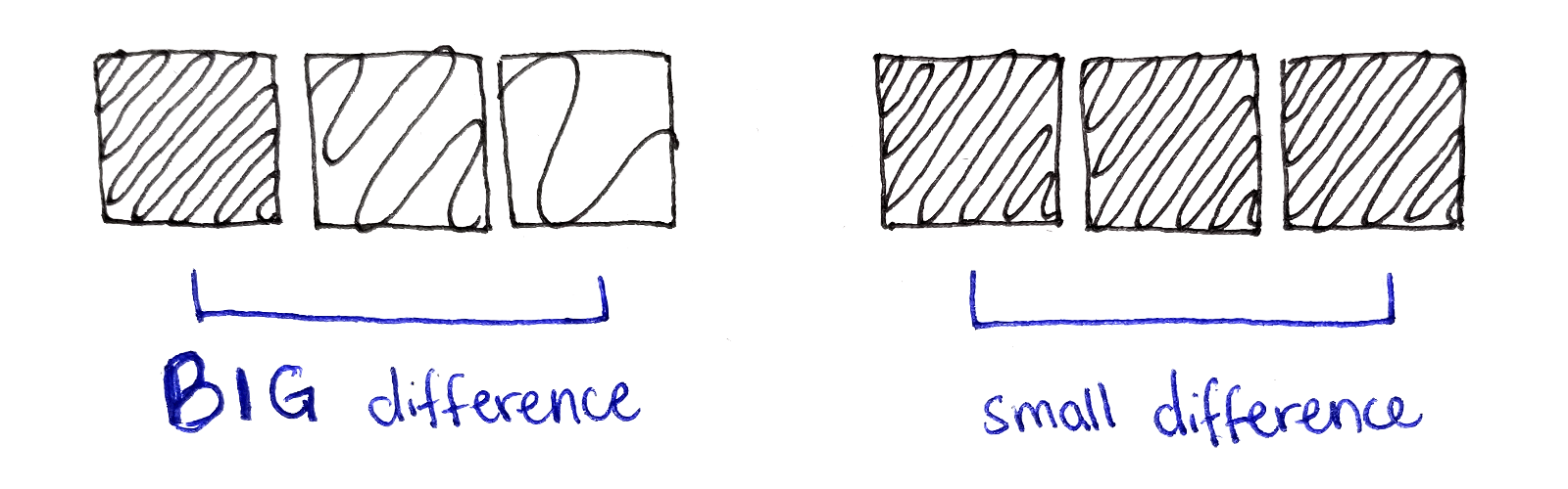
However, after a seam is removed, we will have to consider pixels that were not adjacent before but are adjacent now. So, start by defining the concept of a color difference between two arbitrary pixels $p_0$ and $p_1$:
\[\begin{aligned} D[p_0, p_1] &= D[(x_0, y_0), (x_1, y_1)] \\ &= (R_{p_0} - R_{p_1})^2 + (G_{p_0} - G_{p_1})^2 + (B_{p_0} - B_{p_1})^2 \end{aligned}\]Next, we have to consider which pixels are brought together by the removal of a particular pixel. This depends on if the current pixel is connected to a seam on the top-left, top or top-right. For example, if the current pixel connects to the seam on the top-left, then the following pixels are now touching where they weren’t before:
The pixel to the left of the current one, with coordinates $(x-1, y)$, is now touching the pixel to the right of the current one, with coordinates $(x+1, y)$.
The pixel above the current one, with coordinates $(x, y-1)$, is now touching the pixel to the left of the current one, with coordinates $(x-1, y)$.
These new edges are illustrated in the diagram below, along with the new edges formed when connecting to other seams.
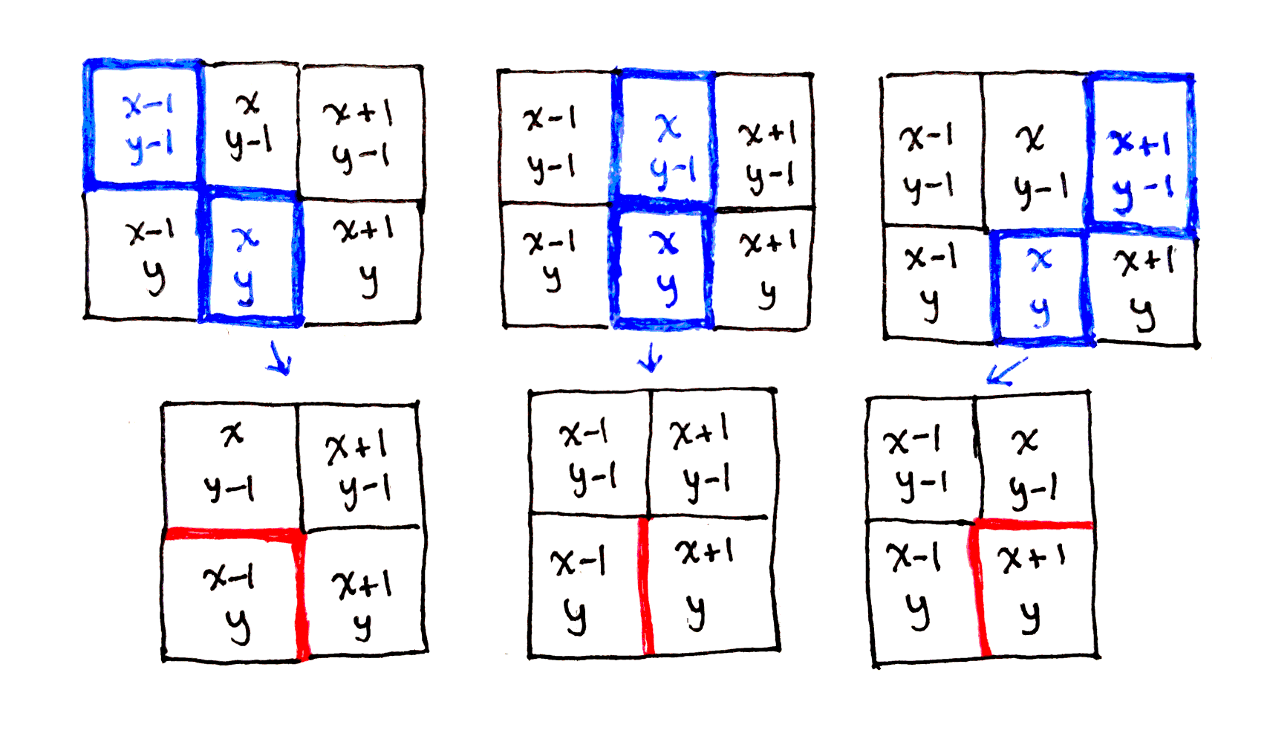
Because these two pairs of pixels will be touching after the seam removal, we compare the color difference between each pair of pixels. Note that we only consider new edges involving pixels in the current row, as the previous row is accounted for when performing these calculations for the previous row.
That means, for the case where we connect to the top-left seam, the new cost is the color difference between pixels $(x-1, y)$ and $(x+1,y)$ along with the color difference between pixels $(x, y-1)$ and $(x-1, y)$. We call this cost $C_L(x, y)$.
Similarly, we have costs $C_U(x, y)$ for when connecting to the top seam and $C_R(x, y)$ for when connecting to the top-right seam. So, instead of having a single energy associated with each pixel, we now have three costs:
\[\begin{aligned} C_L(x, y) &= D[(x - 1, y), (x + 1, y)] + D[(x, y - 1), (x - 1, y)] \\ C_U(x, y) &= D[(x - 1, y), (x + 1, y)] \\ C_R(x, y) &= D[(x - 1, y), (x + 1, y)] + D[(x, y - 1), (x + 1, y)] \\ \end{aligned}\]Notice how, because the current pixel is removed in all three cases, the first term appears in all three equations. The pixels to the left and right of the current pixel are always pushed together.
What the paper doesn’t explain is how to handle the literal edge cases in the image: the top row and the left and right columns. This is typical of many research papers, as the high-level concepts are the focus of the paper. I’ve chosen to handle these edge cases in a particular way, but I can’t guarantee that’s the best way to go about handling these cases.
First, the top row. The top row cannot connect to a previous row, so it makes no sense to consider what happens in such a case. Instead, only the effect of removing the current pixel and therefore connecting the left and right pixels together is considered. This means calculating $C_U$ as above, and $C_L$ and $C_R$ can be initialized to any arbitrary value for the top row. The latter two values will be ignored in the seam finding part of the algorithm:
\[\begin{aligned} C_L(x, 0) &= 0 \\ C_U(x, 0) &= D[(x - 1, 0), (x + 1, 0)] \\ C_R(x, 0) &= 0 \\ \end{aligned}\]The left and right columns are also tricky to handle, as it doesn’t make sense to consider a pixel to the left or right, respectively, of the current pixel. I’ve chosen to handle these cases by replacing references to the left pixel with the current pixel for the left edge, and similarly for the right edge.
For example, the three costs for the left edge become:
\[\begin{aligned} C_L(0, y) &= D[(0, y), (1, y)] + D[(0, y - 1), (0, y)] \\ C_U(0, y) &= D[(0, y), (1, y)] \\ C_R(0, y) &= D[(0, y), (1, y)] + D[(0, y - 1), (1, y)] \\ \end{aligned}\]This is the same as extending the image on each of the left and right edges by one pixel, copying over the nearest column when doing so.
The recurrence relation works mostly the same as before. We associate with each pixel the energy of the lowest-energy seam ending at that pixel. To compute this value, we look at the seams on the top-left, top and top-right of the current pixel, as the current pixel can continue a seam ending at any of those locations.
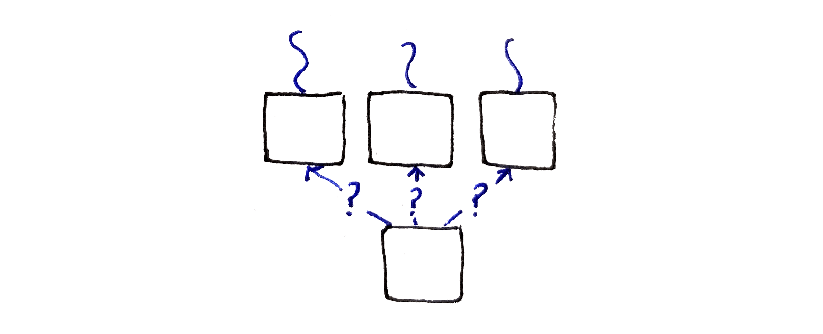
Unlike before, each choice of seam to continue brings different pixels together if that seam were to be removed. This means we have to consider a different cost in each case. For example, if we’re continuing the seam from the top-left pixel, we have to consider the cost $C_L$. Finally, we choose the lowest-energy option out of all of these.
\[\begin{aligned} M(x, y) &= \min \begin{cases} M(x - 1, y - 1) + C_L(x, y) \\ M(x, y - 1) + C_U(x, y) \\ M(x + 1, y - 1) + C_R(x, y) \end{cases} \end{aligned}\]Again, the top row has to be handled specially. It doesn’t make sense to think about connecting to another seam on from the previous row. Instead, we only look at the effect of removing the current pixel, which I described in the last section as being captured by $C_U$:
\[\begin{aligned} M(x, 0) &= C_U(x, 0) \end{aligned}\]When considering the left and right edges, we simply ignore the part of the minimization that corresponds to connecting to the top-left or top-right seams respectively.
I won’t show any example Python code here, because the majority of the algorithm is the same as what I presented in my previous post. The main differences are:
Instead of computing a single energy value for each pixel, three cost values are computed for each pixel.
The main loop in the algorithm performs a different calculation that incorporates these three cost values.
If you want to play around with my implementation and look at the C code, the forward energy implementation is on Github.
Using the forward energy, it’s possible to resize the arch image much more naturally.

The following animated comparison shows shows the result of the resizing using the backward and forward energy. The forward energy preserves straight lines better and generally resizes different parts of the image more uniformly.

Finally, we can see the improved seam removal process over time:
As an additional test, I tried resizing an image of some geese. I didn’t have much success on resizing this image before, as the seam-carving algorithm mangled the straight lines in the image and destroyed the shape of the geese.

Applying the forward energy yielded a much better result:

The authors of the paper also have a number of comparison images that demonstrate the improvements possible using the forward energy.
Forward energy considers the energy of an image after removing a seam, instead of the current energy of the image. This straightforward modification of the original seam carving algorithm results in more natural content-aware image resizing.
There are two takeaways:
There’s always room for improvement. The authors of the original paper found a method to address the limitations of their original findings.
When translating a research paper into an actual implementation, there are usually gaps not covered by the paper. It’s important to make intelligent guesses in order to fill in those gaps.
Hopefully, this makes research papers more accessible. Perhaps someone can implement the extension to videos!