Sep 8, 2020 • Avik Das
The reason I wrote my last two posts on WebGL is because I want to write about my undergraduate research from my time at college. My original paper was written with a bunch of messy C++ code, and I want to do two things:
Make the concepts behind my research more accessible.
Make the results from my research available to people without needing to compile and install additional software. That means WebGL!
Today, I’ll start with some background material: curves and moving frames. While you don’t need to install new software to play with the demos, you will at least need a sufficiently new browser that supports WebGL and modern Javascript features (like modules).
When you describe a curve in any number of dimensions, there are two important properties involved:
The tangent vector at a given point, describing where the curve is headed from that point.
The normal vector at a given point, perpendicular to the tangent. In certain cases, which I’ll talk about more below, the normal describes where the tangent is headed from that point.
Intuitively, the tangent points along the curve, and the normal points away from it.
If you’re familiar with calculus, you may notice I’m describe rates of change, meaning derivatives. Indeed, based on the above definitions, the tangent is simply the derivative of the curve with respect to position and the normal is the derivative of the tangent! This also means, if we have a bunch of discrete points that define a curve, we can approximate these derivatives using finite differences:
\[\begin{alignat}{2} \vec{\mathbf{t}}(t) &= \frac{\mathrm{d}\vec{\mathbf{x}}}{\mathrm{d}t} &\approx \frac{\vec{\mathbf{x}}(t + h) - \vec{\mathbf{x}}(t - h)}{2h} \\ \vec{\mathbf{n}}(t) &= \frac{\mathrm{d}\vec{\mathbf{t}}}{\mathrm{d}t} &\approx \frac{\vec{\mathbf{t}}(t + h) - \vec{\mathbf{t}}(t - h)}{2h} \end{alignat}\](All of this is subtly wrong, but I’ll talk later about what’s wrong and how to fix it.)
Take the surrounding points, find their difference, then divide by the distance between the points. The closer the discrete points, the better the approximation. The same goes for the normal, but this time calculating the differences between the surrounding tangents.
Because these two vectors are rates of change, they have magnitude describing how fast the curve or the tangent are changing. For our purposes, however, we only care about the direction of the change. But, the magnitude of the normal will give us some insight, so in the following interactive demo, I’ve plotted:
You’ll notice that the approximation gets better—the tangent and normal point in the directions you intuitively expect—with more samples along the curve. This is because the step size, the $h$ in the above formulas, gets smaller.
The other very important observation is how the normal behaves around the middle of the curve. In the middle is the inflection point, the point where the curve switches from curving in one direction to curving in the other direction. At that point, the curve approximates a straight line, meaning the tangent is not changing direction and the normal is essentially the zero vector.
This also means the normal points down on one side of the inflection point, getting smaller and smaller until it starts getting bigger on the other side. The unit-length normal vector suddenly switches directions, which will come back to bite us shortly.
I said above my explanation of the tangent and normal are subtly wrong. The problem is the tangent and the normal should be inherent properties of the curve, regardless of how you represent it.
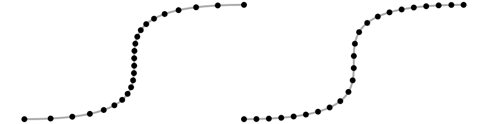
That means the tangent and the normal are generally represented based on the arc-length parameterization, and the calculations above only work under this parameterization. Intuitively, we need to sample points evenly spaced along the curve, as seen in the visualization below:
On the left, because of how the curve is defined (as a cubic Bézier curve), sampling at “evenly-spaced” intervals causes our samples to bunch up in the middle. This basically means the curve is moving slower near the middle and faster near the ends. What we actually want to do is pick samples that end up evenly-spaced, like on the right side. We want curve to move at the same speed all throughout.
Unfortunately, generating the arc-length parameterization is not easy to do in general. Luckily, for the applications I’m talking about, it doesn’t matter! If we take enough samples, the samples will be close enough that the finite differences approximation will work out. One caveat is that when computing the normal, you need to normalize the tangent vectors first. Remember, in the arc-length parameterization, samples are evenly-spaced, meaning the tangent is always a fixed length. Only then is the normal the derivative of the tangent.
If you want to render a 1D curve as a 3D model, you need an orientation for the various cross sections. For example, if you’re describing a snake as a curve, you need a direction that counts as “up”. You can see this in the image below:
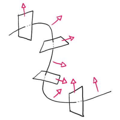
So, how do you define the orientation of the cross sections? Well, you need one vector that’s perpendicular to the tangent. That vector doesn’t need to be your “up” vector, as long as it’s always related in the same way to the “up” vector on each cross section. And, we have such a vector: the normal!
This observation is the key to the Frenet-Serret frame. To define an oriented plane in which a cross section will lie:
Start with the unit-length normal vector at the point in question. This is our reference vector.
Because the tangent is perpendicular to the cross section’s plane, you can take the cross product of the tangent and the normal ($\hat{\mathbf{t}} \times \hat{\mathbf{n}}$) to get another unit-length vector on the cross section’s plane. In fact, this vector will be perpendicular to the normal vector. Call this new vector $\hat{\mathbf{b}}$ for “binormal” vector.
Now, you have two vectors, $\hat{\mathbf{n}}$ and $\hat{\mathbf{b}}$ that define your plane, and you can orient your cross section accordingly. For example, you might just make the binormal vector your “up” direction.
Unfortunately, this is where we run into the problem with the normal vector suddenly flipping directions. If the curve has an inflection point, then the cross section will suddenly rotate $180^{\circ}$. You can see that in the following demo:
(Link to screenshot if your browser isn’t new enough.)
Luckily, we can fix this problem using the Rotation Minimizing Frame or RMF. The paper Computation of Rotation Minimizing Frames goes over both the definition and an efficient calculation of the RMF, but intuitively:
Instead of using the normal as the reference vector, we want to choose a reference vector that doesn’t rotate around the tangent so much. In fact, formally, the ideal reference vector’s first derivative is in the same direction as the tangent, meaning the reference vector only moves along the tangent.
And, in order to be a reference vector for the cross section we care about, the reference vector has to remain perpendicular to the tangent.
As the paper explains, the RMF is defined by a set of Ordinary Differential Equations (ODEs), so finding the true solution is not trivial in general. Luckily, the algorithm presented in the paper is really easy to implement (I won’t go over the details here) and approximates the true solution really well. You can see how well the RMF behaves in the next demo:
(Link to screenshot if your browser isn’t new enough.)
The only caveat here is we need an initial frame to start off the process. In the above demo, I’ve used the Frenet-Serret frame at $t = 0$, but in real applications, you’ll probably want to manually specify the initial frame. This is especially important for curves where the the normal is zero at the beginning of the curve because the curve starts off like a straight line.
A curious thing can happen if the curve is a closed loop that doesn’t lie on one plane. Take a look at the following curve:
(Link to screenshot if your browser isn’t new enough.)
Even though the cross sections are created using Rotation Minimizing Frames, the starting and ending cross sections don’t line up with each other. In fact, I created this curve so that the starting and ending frames are exactly $180^{\circ}$ apart!
I’ll talk more about why this happens in later articles, as this very phenomenon was the subject of my research.
If you’re curious, I used the following technologies for the visualizations in this article:
Preact - a React-like DOM rendering library. Used for the 2D visualization, which reacts to the sliders.
three.js - a 3D rendering library that makes it easy to render WebGL content. It helped me to first understand WebGL (I even initially wrote all my rendering from scratch) before I started using an abstraction over it.
Unpkg for making it easy to import libraries from a CDN.
Thanks to Ty Terdan