
Jun 24, 2019 • Avik Das
Machine learning requires many sophisticated algorithms to learn from existing data, then apply the learnings to new data. Dynamic programming turns up in many of these algorithms. This may be because dynamic programming excels at solving problems involving “non-local” information, making greedy or divide-and-conquer algorithms ineffective.
In this article, I’ll explore one technique used in machine learning, Hidden Markov Models (HMMs), and how dynamic programming is used when applying this technique. After discussing HMMs, I’ll show a few real-world examples where HMMs are used.
This article is part of an ongoing series on dynamic programming. If you need a refresher on the technique, see my graphical introduction to dynamic programming.
(I gave a talk on this topic at PyData Los Angeles 2019, if you prefer a video version of this post.)
A Hidden Markov Model deals with inferring the state of a system given some unreliable or ambiguous observations from that system. One important characteristic of this system is the state of the system evolves over time, producing a sequence of observations along the way. There are some additional characteristics, ones that explain the Markov part of HMMs, which will be introduced later. By incorporating some domain-specific knowledge, it’s possible to take the observations and work backwards to a maximally plausible ground truth.
As a motivating example, consider a robot that wants to know where it is. Unfortunately, its sensor is noisy, so instead of reporting its true location, the sensor sometimes reports nearby locations. These reported locations are the observations, and the true location is the state of the system.
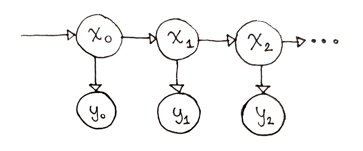
An HMM consists of a few parts. First, there are the possible states $s_i$, and observations $o_k$. These define the HMM itself. An instance of the HMM goes through a sequence of states, $x_0, x_1, …, x_{n-1}$, where $x_0$ is one of the $s_i$, $x_1$ is one of the $s_i$, and so on. Each state produces an observation, resulting in a sequence of observations $y_0, y_1, …, y_{n-1}$, where $y_0$ is one of the $o_k$, $y_1$ is one of the $o_k$, and so on.
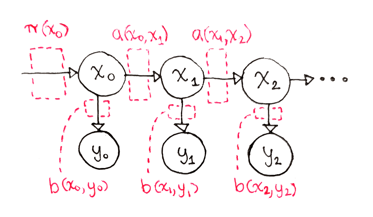
Next, there are parameters explaining how the HMM behaves over time:
There are the Initial State Probabilities. For each possible state $s_i$, what is the probability of starting off at state $s_i$? These probabilities are denoted $\pi(s_i)$.
There is the State Transition Matrix, defining how the state changes over time. If the system is in state $s_i$ at some time, what is the probability of ending up at state $s_j$ after one time step? These probabilities are called $a(s_i, s_j)$.
There is the Observation Probability Matrix. If the system is in state $s_i$, what is the probability of observing observation $o_k$? These probabilities are called $b(s_i, o_k)$.
The last two parameters are especially important to HMMs. The second parameter is set up so, at any given time, the probability of the next state is only determined by the current state, not the full history of the system. This is the “Markov” part of HMMs. The third parameter is set up so that, at any given time, the current observation only depends on the current state, again not on the full history of the system.
The primary question to ask of a Hidden Markov Model is, given a sequence of observations, what is the most probable sequence of states that produced those observations? We can answer this question by looking at each possible sequence of states, picking the sequence that maximizes the probability of producing the given observations. As we’ll see, dynamic programming helps us look at all possible paths efficiently.
In dynamic programming problems, we typically think about the choice that’s being made at each step. In my previous article about seam carving, I discussed how it seems natural to start with a single path and choose the next element to continue that path. That choice leads to a non-optimal greedy algorithm. Instead, the right strategy is to start with an ending point, and choose which previous path to connect to the ending point. We’ll employ that same strategy for finding the most probably sequence of states.
The algorithm we develop in this section is the Viterbi algorithm.
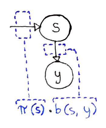
Let’s start with an easy case: we only have one observation $y$. Which state mostly likely produced this observation? For a state $s$, two events need to take place:
We have to start off in state $s$, an event whose probability is $\pi(s)$.
That state has to produce the observation $y$, an event whose probability is $b(s, y)$.
Based on the “Markov” property of the HMM, where the probability of observations from the current state don’t depend on how we got to that state, the two events are independent. This allows us to multiply the probabilities of the two events. So, the probability of observing $y$ on the first time step (index $0$) is:
With the above equation, we can define the value $V(t, s)$, which represents the probability of the most probable path that:
Has $t + 1$ states, starting at time step $0$ and ending at time step $t$.
Ends in state $s$.
Produces the first $t + 1$ observations given to us.
So far, we’ve defined $V(0, s)$ for all possible states $s$.
If we only had one observation, we could just take the state $s$ with the maximum probability $V(0, s)$, and that’s our most probably “sequence” of states. But if we have more observations, we can now use recursion.
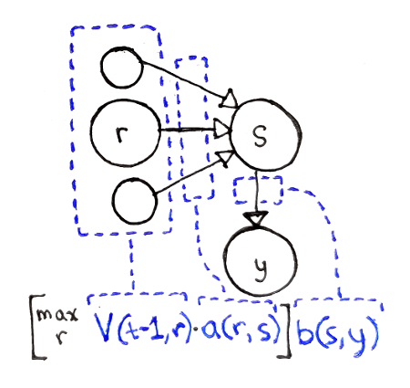
Let’s say we’re considering a sequence of $t + 1$ observations. We don’t know what the last state is, so we have to consider all the possible ending states $s$. We also don’t know the second to last state, so we have to consider all the possible states $r$ that we could be transitioning from. This means we need the following events to take place:
We need to end at state $r$ at the second-to-last step in the sequence, an event with probability $V(t - 1, r)$.
We have to transition from some state $r$ into the final state $s$, an event whose probability is $a(r, s)$.
The final state has to produce the observation $y$, an event whose probability is $b(s, y)$.
All these probabilities are independent of each other. As a result, we can multiply the three probabilities together. This probability assumes that we have $r$ at the second-to-last step, so we now have to consider all possible $r$ and take the maximum probability:
This defines $V(t, s)$ for each possible state $s$.
Notice that the observation probability depends only on the last state, not the second-to-last state. This means we can extract out the observation probability out of the $\max$ operation.
Another important characteristic to notice is that we can’t just pick the most likely second-to-last state, that is we can’t simply maximize $V(t - 1, r)$. It may be that a particular second-to-last state is very likely. However, if the probability of transitioning from that state to $s$ is very low, it may be more probable to transition from a lower probability second-to-last state into $s$.
As a recap, our recurrence relation is formally described by the following equations:
\[\begin{aligned} V(0, s) & = \pi(s) \cdot b(s, y) \\ V(t, s) & = \bigg[ \max_r V(t - 1, r) \cdot a(r, s) \bigg] \cdot b(s, y) \end{aligned}\]This recurrence relation is slightly different from the ones I’ve introduced in my previous posts, but it still has the properties we want:
The recurrence relation has integer inputs. Technically, the second input is a state, but there are a fixed set of states. We can assign integers to each state, though, as we’ll see, we won’t actually care about ordering the possible states.
The final answer we want is easy to extract from the relation. We look at all the values of the relation at the last time step and find the ending state that maximizes the path probability.
The relation depends on itself.
Looking at the recurrence relation, there are two parameters. The first parameter $t$ spans from $0$ to $T - 1$, where $T$ is the total number of observations. This is because there is one hidden state for each observation.
The second parameter $s$ spans over all the possible states, meaning this parameter can be represented as an integer from $0$ to $S - 1$, where $S$ is the number of possible states. Each integer represents one possible state.
This means we can lay out our subproblems as a two-dimensional grid of size $T \times S$. The columns represent the set of all possible ending states at a single time step, with each row being a possible ending state.
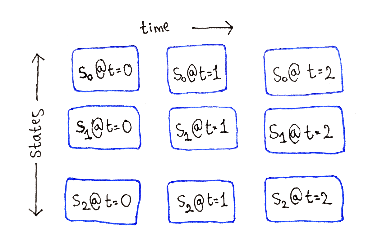
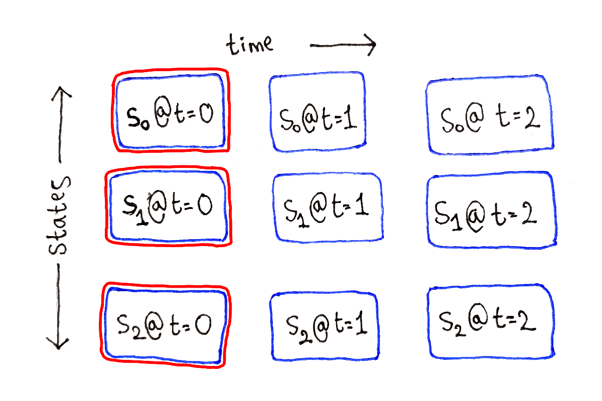
At time $t = 0$, that is at the very beginning, the subproblems don’t depend on any other subproblems. These are our base cases.
For any other $t$, each subproblem depends on all the subproblems at time $t - 1$, because we have to consider all the possible previous states.
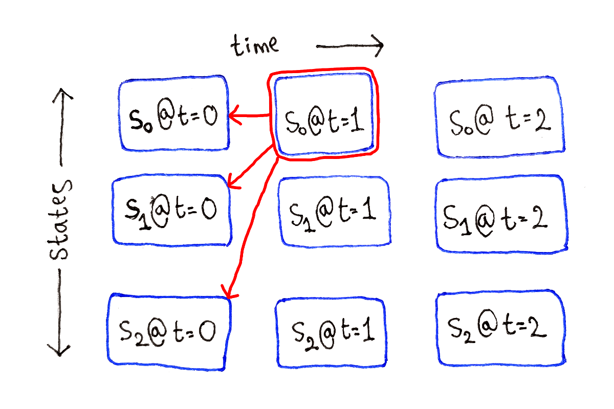
This process is repeated for each possible ending state at each time step.
Like in the previous article, I’m not showing the full dependency graph because of the large number of dependency arrows.
From the above analysis, we can see we should solve subproblems in the following order:
Because each time step only depends on the previous time step, we should be able to keep around only two time steps worth of intermediate values. However, because we want to keep around back pointers, it makes sense to keep around the results for all subproblems.
The following implementation borrows a great deal from the similar seam carving implementation from my last post, so I’ll skip ahead to using back pointers.
First, we need a representation of our HMM, with the three parameters we defined at the beginning of the post. The parameters are:
p representing the initial probabilities $\pi(s)$.a representing the state transition matrix $a(r, s)$.b representing the observation probability matrix $b(s, y)$.As a convenience, we also store a list of the possible states, which we will loop over frequently.
class HMM:
    def __init__(self, p, a, b):
        self.possible_states = p.keys()
        self.p = p
        self.a = a
        self.b = b

# The following is an example. We'll define a more meaningful HMM later.
hmm = HMM(
    # initial state probabilities
    { 's0': 0.6, 's1': 0.4 },

    # state transition matrix
    {
        's0': { 's0': 0.6, 's1': 0.4 },
        's1': { 's0': 0.4, 's1': 0.6 }
    },

    # observation probability matrix
    {
        's0': { 'y0': 0.8, 'y1': 0.2 },
        's1': { 'y0': 0.2, 'y1': 0.8 }
    }
)
Just like in the seam carving implementation, we’ll store elements of our two-dimensional grid as instances of the following class. The class simply stores the probability of the corresponding path (the value of $V$ in the recurrence relation), along with the previous state that yielded that probability.
class PathProbabilityWithBackPointer:
    def __init__(self, probability, previous_state=None):
        self.probability = probability
        self.previous_state = previous_state
With all this set up, we start by calculating all the base cases. This means calculating the probabilities of single-element paths that end in each of the possible states. Here, observations is a list of strings representing the observations we’ve seen.
path_probabilities = []

# Initialize the first time step of path probabilities based on the initial
# state probabilities. There are no back pointers in the first time step.
path_probabilities.append({
    possible_state: PathProbabilityWithBackPointer(
        hmm.p[possible_state] *
        hmm.b[possible_state][observations[0]])
    for possible_state in hmm.s
})
Next comes the main loop, where we calculate $V(t, s)$ for every possible state $s$ in terms of $V(t - 1, r)$ for every possible previous state $r$.
# Skip the first time step in the following loop.
for t in range(1, len(observations)):
    observation = observations[t]

    latest_path_probabilities = {}
    for possible_state in hmm.possible_states:
        max_previous_state = max(
            hmm.possible_states,
            key=lambda s_i: (
                path_probabilities[t - 1][s_i].probability *
                hmm.a[s_i][possible_state]
            )
        )

        max_path_probability = PathProbabilityWithBackPointer(
            hmm.b[possible_state][observation] *
            path_probabilities[t - 1][max_previous_state].probability *
            hmm.a[max_previous_state][possible_state],
            max_previous_state
        )

        latest_path_probabilities[possible_state] = max_path_probability

    path_probabilities.append(latest_path_probabilities)
After finishing all $T - 1$ iterations, accounting for the fact the first time step was handled before the loop, we can extract the end state for the most probable path by maximizing over all the possible end states at the last time step.
max_path_end_state = max(
    hmm.possible_states,
    key=lambda s: path_probabilities[-1][s].probability
)
Finally, we can now follow the back pointers to reconstruct the most probable path.
path = []
path_step_state = max_path_end_state
for t in range(len(path_probabilities) - 1, -1, -1):
    path.append(path_step_state)

    path_step_state = \
        path_probabilities[t][path_step_state].previous_state

path.reverse()
Try testing this implementation on the following HMM.
hmm = HMM(
    # initial state probabilities
    { 's0': 0.8, 's1': 0.1, 's2': 0.1 },

    # state transition matrix
    {
        's0': { 's0': 0.9, 's1': 0.1, 's2': 0.0 },
        's1': { 's0': 0.0, 's1': 0.0, 's2': 1.0 },
        's2': { 's0': 0.0, 's1': 0.0, 's2': 1.0 }
    },

    # observation probability matris
    {
        's0': { 'y0': 1.0, 'y1': 0.0 },
        's1': { 'y0': 1.0, 'y1': 0.0 },
        's2': { 'y0': 0.0, 'y1': 1.0 }
    }
)
In this HMM, the third state s2 is the only one that can produce the observation y1. Additionally, the only way to end up in state s2 is to first get to state s1. Starting with observations ['y0', 'y0', 'y0'], the most probable sequence of states is simply ['s0', 's0', 's0'] because it’s not likely for the HMM to transition to to state s1.
However, if you then observe y1 at the fourth time step, the most probable path changes. You know the last state must be s2, but since it’s not possible to get to that state directly from s0, the second-to-last state must be s1. This means the most probable path is ['s0', 's0', 's1', 's2'].
From the dependency graph, we can tell there is a subproblem for each possible state at each time step. Because we have to save the results of all the subproblems to trace the back pointers when reconstructing the most probable path, the Viterbi algorithm requires $O(T \times S)$ space, where $T$ is the number of observations and $S$ is the number of possible states.
We have to solve all the subproblems once, and each subproblem requires iterating over all $S$ possible previous states. Thus, the time complexity of the Viterbi algorithm is $O(T \times S^2)$.
Finding the most probable sequence of hidden states helps us understand the ground truth underlying a series of unreliable observations. This comes in handy for two types of tasks:
Filtering, where noisy data is cleaned up to reveal the true state of the world. Determining the position of a robot given a noisy sensor is an example of filtering.
Recognition, where indirect data is used to infer what the data represents.
Let’s look at some more real-world examples of these tasks:
Speech recognition. Also known as speech-to-text, speech recognition observes a series of sounds. These sounds are then used to infer the underlying words, which are the hidden states.
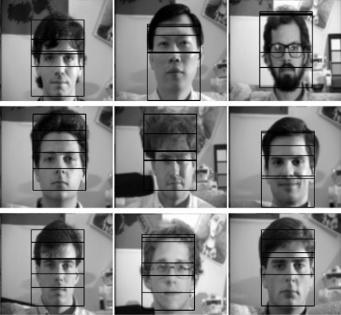
Face detection. In order to find faces within an image, one HMM-based face detection algorithm observes overlapping rectangular regions of pixel intensities. These intensities are used to infer facial features, like the hair, forehead, eyes, etc. The features are the hidden states, and when the HMM encounters a region like the forehead, it can only stay within that region or transition to the “next” state, in this case the eyes. If all the states are present in the inferred state sequence, then a face has been detected. See Face Detection and Recognition using Hidden Markov Models by Nefian and Hayes.
Computational biology. HMMs have found widespread use in computational biology. One problem is to classify different regions in a DNA sequence. The elements of the sequence, DNA nucleotides, are the observations, and the states may be regions corresponding to genes and regions that don’t represent genes at all. For a survey of different applications of HMMs in computation biology, see Hidden Markov Models and their Applications in Biological Sequence Analysis.
As in any real-world problem, dynamic programming is only a small part of the solution. Most of the work is getting the problem to a point where dynamic programming is even applicable. In this section, I’ll discuss at a high level some practical aspects of Hidden Markov Models I’ve previously skipped over.
Real-world problems don’t appear out of thin air in HMM form. To apply the dynamic programming approach, we need to frame the problem in terms of states and observations. This is known as feature extraction and is common in any machine learning application.
In the above applications, feature extraction is applied as follows:
In speech recognition, the incoming sound wave is broken up into small chunks and the frequencies extracted to form an observation. For information, see The Application of Hidden Markov Modelsin Speech Recognition by Gales and Young.
In face detection, looking at a rectangular region of pixels and directly using those intensities makes the observations sensitive to noise in the image. Furthermore, many distinct regions of pixels are similar enough that they shouldn’t be counted as separate observations. To combat these shortcomings, the approach described in Nefian and Hayes 1998 (linked in the previous section) feeds the pixel intensities through an operation known as the Karhunen–Loève transform in order to extract only the most important aspects of the pixels within a region.
In computational biology, the observations are often the elements of the DNA sequence directly. Sometimes, however, the input may be elements of multiple, possibly aligned, sequences that are considered together.
All this time, we’ve inferred the most probable path based on state transition and observation probabilities that have been given to us. But how do we find these probabilities in the first place? Determining the parameters of the HMM is the responsibility of training.
I won’t go into full detail here, but the basic idea is to initialize the parameters randomly, then use essentially the Viterbi algorithm to infer all the path probabilities. These probabilities are used to update the parameters based on some equations. This procedure is repeated until the parameters stop changing significantly.
The concept of updating the parameters based on the results of the current set of parameters in this way is an example of an Expectation-Maximization algorithm. When applied specifically to HMMs, the algorithm is known as the Baum-Welch algorithm.
Machine learning permeates modern life, and dynamic programming gives us a tool for solving some of the problems that come up in machine learning. In particular, Hidden Markov Models provide a powerful means of representing useful tasks. To make HMMs useful, we can apply dynamic programming.
The last couple of articles covered a wide range of topics related to dynamic programming. Let me know what you’d like to see next! Is there a specific part of dynamic programming you want more detail on? Or would you like to read about machine learning specifically? Let me know so I can focus on what would be most useful to cover.